Shapes in multi-objective programming

Package gMOIP has different features for plotting different shapes in 3D.

We define the sets \(\mathbb{R}_{>} = \{ z\in \mathbb{R} \mid z > 0\}\), \(\mathbb{R}_{\geqq} = \{ z\in \mathbb{R} \mid z \geqq 0\}\) and \(\mathbb{R}_{\geqslant} = \{ z\in \mathbb{R} \mid z \geqslant 0\}\):

The non-dominated set (red points are non-dominated and black dominated):

We may also add dominance cones and the hull:

Note the area between the hull and the cones is the search area where further nondominated points may be found.

Another example with more unsupported points:

We may also plot reverse dominance cones:

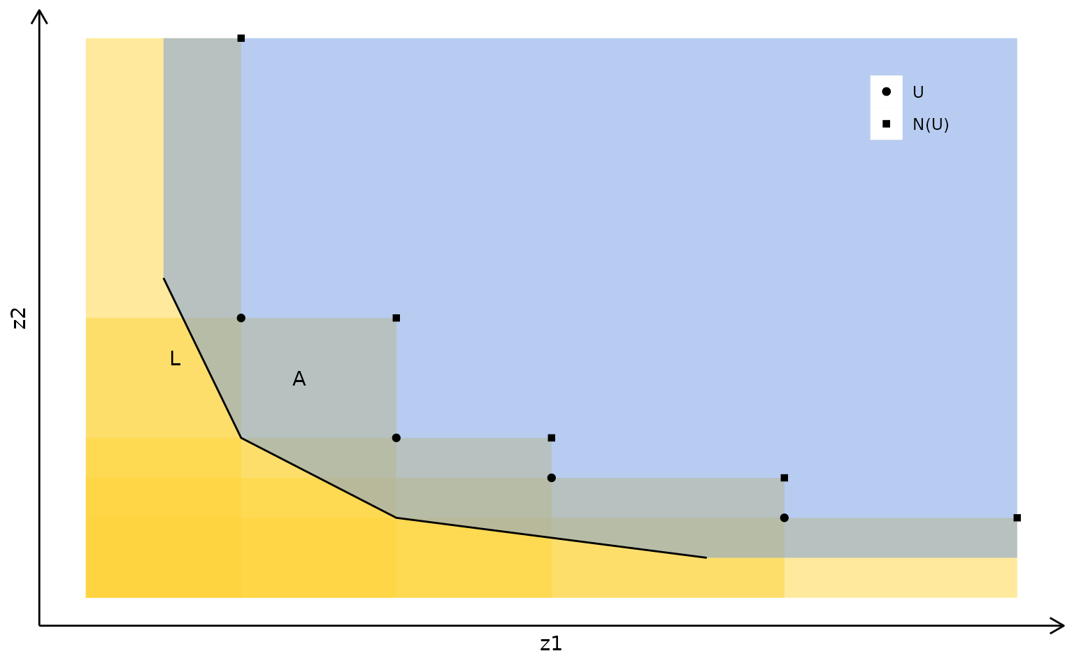
Given a lower bound set \(L\) (the line segments) and an upper bound set \(U\) with local upper bounds \(N(U)\), the search region \(A\) is given by the closure of the gray area:

A lower bound set (solid and dashed lines) partially dominated by the upper bound set. The dominated area of the lower bound set is represented by the dashed lines. Three disjoint subproblems are created in the objective space by applying objective branching on \(y1\), \(y2\) and \(y3\), represented by the red circles. The constraints added when applying objective branching are represented by the dotted lines. A new non-dominated point feasible for the corresponding problem can only be found in one of these subproblems (gray areas):

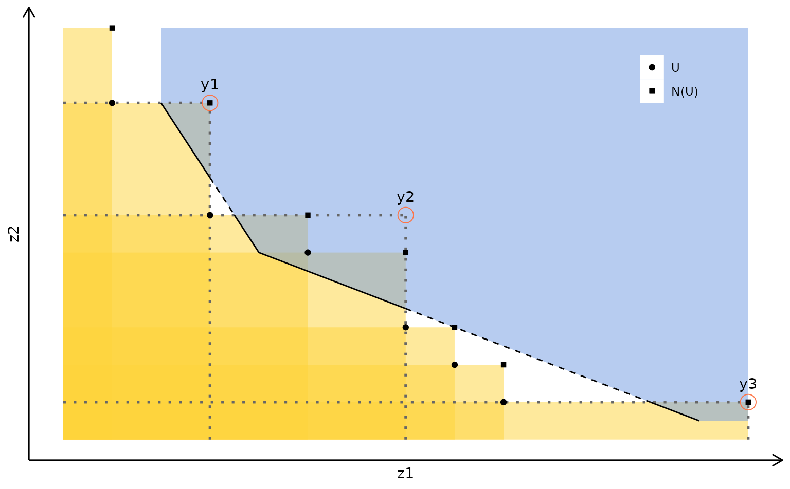
Bi-objective case: The dominated part of the lower bound set is represented by the dashed line. When objective branching is applied on each local upper bound, the search areas (gray) are disjoint:

Three-objective case: The dominated part of the lower bound set is the blue area in the middle. When objective branching is applied on each local upper bound, there are redundancies between the subproblems (each subproblem defines a gray search area). Every point in the red areas is included in the search area of more than one subproblem:

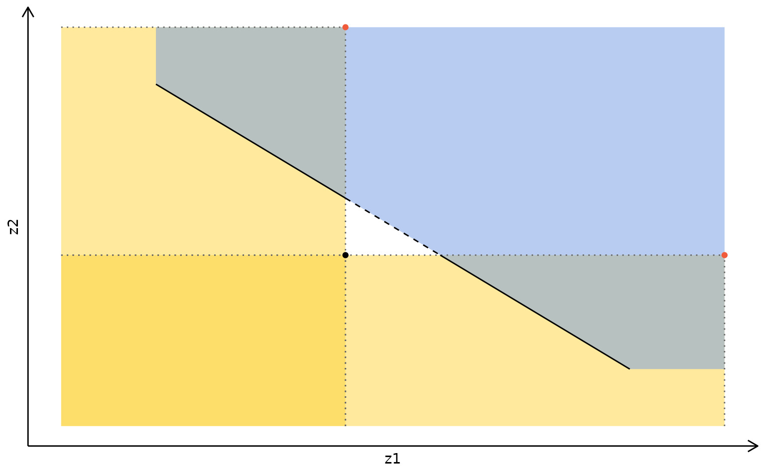
Lower bound set (hyperplane) partially dominated by the upper bound set (black points with red dominance cones). Note the two disjoint search areas above the hyperplane:

Objective branching applied to \(y^1\) and \(y^2\). One subproblem is fully included in the other subproblem:

Another view:

Lars Relund Nielsen

2024-02-21