The gMOIP package can be used to make 2D and 3D plots of
linear programming (LP), integer linear programming (ILP), or mixed
integer linear programming (MILP) models with up to three objectives.
This include the polytope, integer points, ranges and iso profit curve.
Plots of both the solution and criterion space are possible. For
instance the non-dominated (Pareto) set for bi-objective LP/ILP/MILP
programming models.
The package also include an inHull function for checking
if a set of points is inside/at/outside the convex hull of a set of
vertices (for arbitrary dimension).
Finally, the package also contains functions for generating (non-dominated) points in and classifying non-dominated points as supported extreme, supported non-extreme and unsupported.
Installation
Install the latest stable release from CRAN:
install.packages("gMOIP")Alternatively, install the latest development version from GitHub (recommended):
install.packages("devtools")
devtools::install_github("relund/gMOIP")
library(gMOIP)
Single criterion models
We define the model
(could also be minimized) using matrix A and vectors
b and obj:
A <- matrix(c(-3,2,2,4,9,10), ncol = 2, byrow = TRUE)
b <- c(3,27,90)
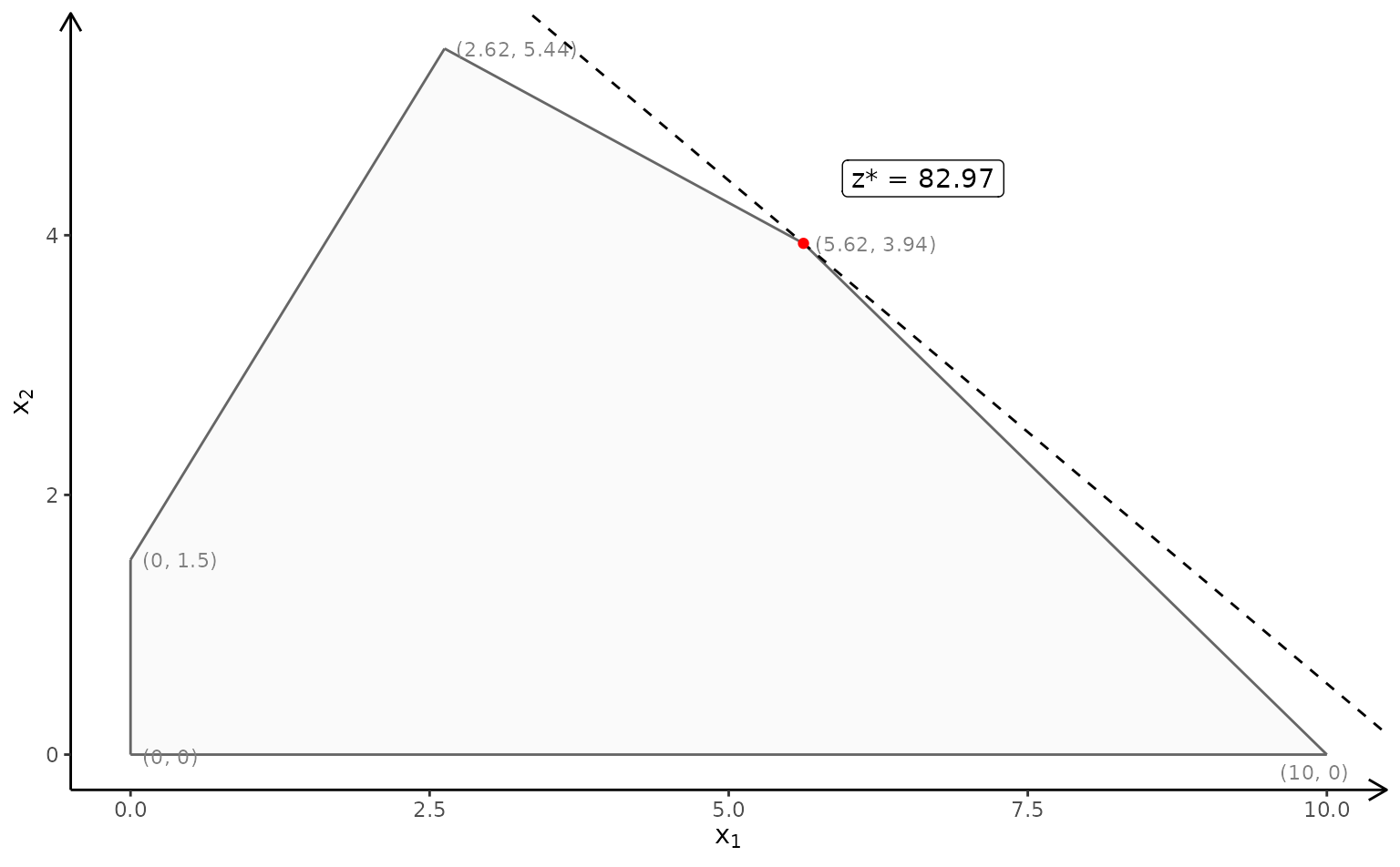
obj <- c(7.75, 10) # coefficients cThe polytope of the LP model with non-negative continuous variables ():
plotPolytope(
   A,
   b,
   obj,
   type = rep("c", ncol(A)),
   crit = "max",
   faces = rep("c", ncol(A)),
   plotFaces = TRUE,
   plotFeasible = TRUE,
   plotOptimum = TRUE,
   labels = "coord"
)
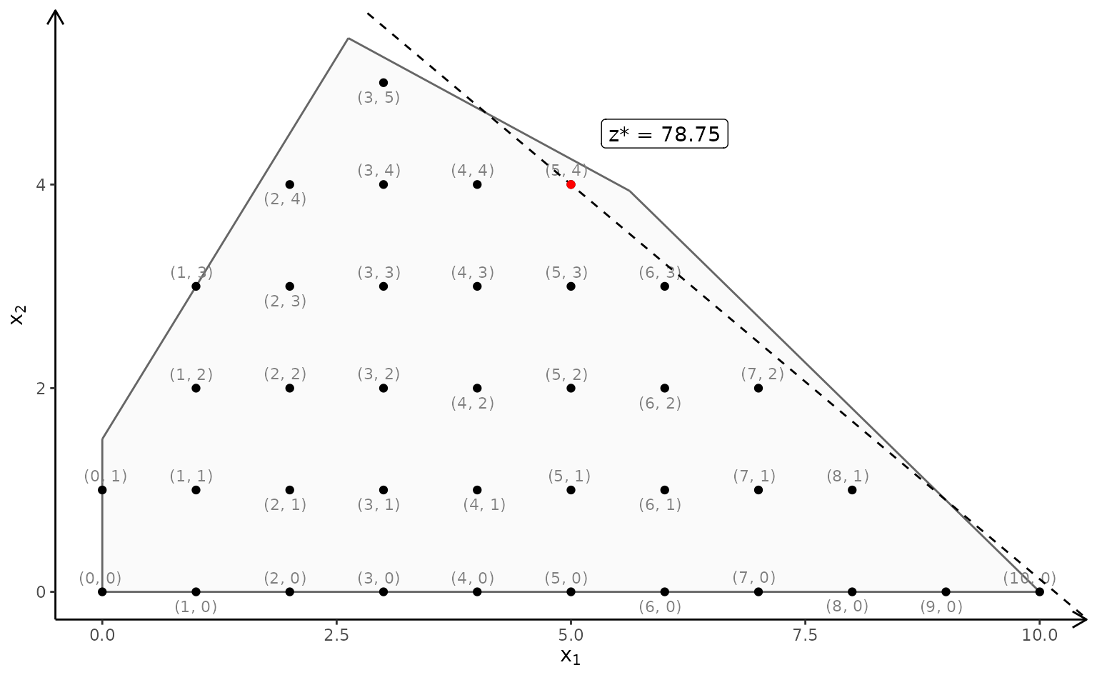
The polytope of the ILP model with LP faces ():
plotPolytope(
   A,
   b,
   obj,
   type = rep("i", ncol(A)),
   crit = "max",
   faces = rep("c", ncol(A)),
   plotFaces = TRUE,
   plotFeasible = TRUE,
   plotOptimum = TRUE,
   labels = "coord"
)
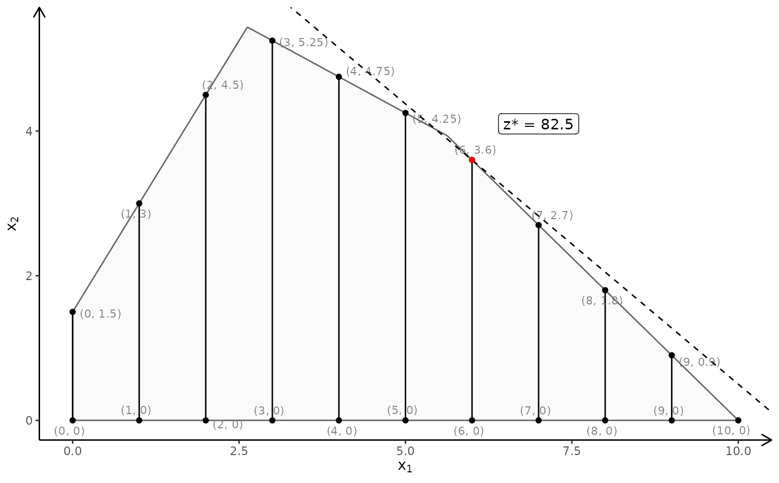
The polytope of the MILP model (first variable integer) with LP faces:
plotPolytope(
   A,
   b,
   obj,
   type = c("i", "c"),
   crit = "max",
   faces = c("c", "c"),
   plotFaces = TRUE,
   plotFeasible = TRUE,
   plotOptimum = TRUE,
   labels = "coord"
)
Three variables
You can do the same with three variables:
A <- matrix( c(
   3, 2, 5,
   2, 1, 1,
   1, 1, 3,
   5, 2, 4
), nc = 3, byrow = TRUE)
b <- c(55, 26, 30, 57)
obj <- c(20, 10, 15)
LP model:
view <- matrix( c(-0.412063330411911, -0.228006735444069, 0.882166087627411, 0, 0.910147845745087,
                  -0.0574885793030262, 0.410274744033813, 0, -0.042830865830183, 0.97196090221405,
                  0.231208890676498, 0, 0, 0, 0, 1), nc = 4)
loadView(v = view)  # set view angle
plotPolytope(A,
             b,
             obj,
             plotOptimum = TRUE,
             labels = "n")
ILP model (here with ILP faces):
view <- matrix( c(-0.412063330411911, -0.228006735444069, 0.882166087627411, 0, 0.910147845745087,
                  -0.0574885793030262, 0.410274744033813, 0, -0.042830865830183, 0.97196090221405,
                  0.231208890676498, 0, 0, 0, 0, 1), nc = 4)
loadView(v = view)  # set view angle
plotPolytope(A,
             b,
             obj,
             type = c("i", "i", "i"),
             plotOptimum = TRUE,
             labels = "n")
MILP model (here with continuous faces):
view <- matrix( c(-0.412063330411911, -0.228006735444069, 0.882166087627411, 0, 0.910147845745087,
                  -0.0574885793030262, 0.410274744033813, 0, -0.042830865830183, 0.97196090221405,
                  0.231208890676498, 0, 0, 0, 0, 1), nc = 4)
loadView(v = view)  # set view angle
plotPolytope(A,
             b,
             obj,
             type = c("i", "i", "c"),
             faces = c("c", "c", "c"),
             plotOptimum = TRUE,
             # plotFaces = FALSE,
             labels = "n")
Bi-objective models
With gMOIP you can also make plots of the criterion
space for bi-objective models (linear programming (LP), integer linear
programming (ILP), or mixed integer linear programming (MILP)).
First let us have a look at bi-objective model with two variables. We define a function for grouping plots of the solution and criterion space:
plotBiObj2D <- function(A, b, obj,
   type = rep("c", ncol(A)),
   crit = "max",
   faces = rep("c", ncol(A)),
   plotFaces = TRUE,
   plotFeasible = TRUE,
   plotOptimum = FALSE,
   labels = "numb",
   addTriangles = TRUE,
   addHull = TRUE)
{
   p1 <- plotPolytope(A, b, type = type, crit = crit, faces = faces, plotFaces = plotFaces,
                      plotFeasible = plotFeasible, plotOptimum = plotOptimum, labels = labels) +
      ggplot2::ggtitle("Solution space")
   p2 <- plotCriterion2D(A, b, obj, type = type, crit = crit, addTriangles = addTriangles,
                         addHull = addHull, plotFeasible = plotFeasible, labels = labels) +
      ggplot2::ggtitle("Criterion space")
   gridExtra::grid.arrange(p1, p2, nrow = 1)
}
Let us define the constraints:
First let us have a look at a LP model (maximize):
obj <- matrix(
   c(7, -10, # first criterion
     -10, -10), # second criterion
   nrow = 2)
plotBiObj2D(A, b, obj, addTriangles = FALSE)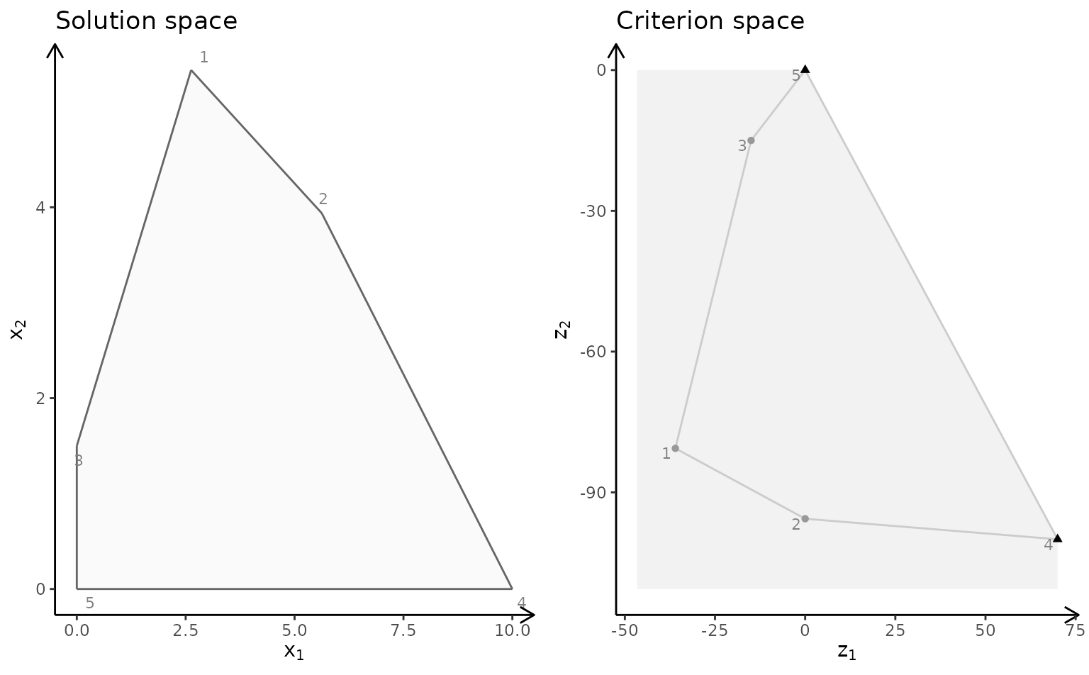
Note the non-dominated (Pareto) set consists of all supported extreme non-dominated points (illustrated with triangles) and the line segments between them.
ILP model (maximize):
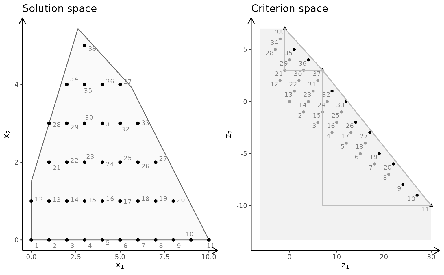
Note the non-dominated set consists of all points in black (with shape supported extreme:triangle, supported non-extreme:round, unsupported:round (not on the border)). The triangles drawn using the extreme non-dominated points illustrate areas where unsupported non-dominated points may be found. A point in the solution space is identified in the criterion space using the same number.
MILP model ( integer) (minimize):
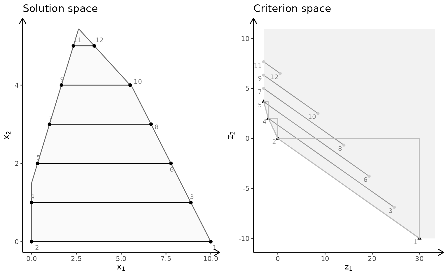
Note the solution space now consists to segments and hence the
non-dominated set may consist of points and segments (open and closed).
Note these segments are not highlighted in the current version of
gMOIP.
Bi-objective models with three variables
We define functions for plotting the solution and criterion space:
plotSol <- function(A, b, type = rep("c", ncol(A)),
                        faces = rep("c", ncol(A)),
                        plotFaces = TRUE, labels = "numb")
{
   loadView(v = view, close = F, zoom = 0.75)
   plotPolytope(A, b, type = type, faces = faces, labels = labels, plotFaces = plotFaces,
                argsTitle3d = list(main = "Solution space"))
}

plotCrit <- function(A, b, obj, crit = "min", type = rep("c", ncol(A)), addTriangles = TRUE,
                     labels = "numb")
{
    plotCriterion2D(A, b, obj, type = type, crit = crit, addTriangles = addTriangles,
                   labels = labels) +
      ggplot2::ggtitle("Criterion space")
}
Four examples are given. A few plots of the solution space are made interactive to illustrate the functionality.
Example 1
We define the model (could also be minimized) with three variables:
Ab <- matrix( c(
   1, 1, 2, 5,
   2, -1, 0, 3,
   -1, 2, 1, 3,
   0, -3, 5, 2
), nc = 4, byrow = TRUE)
A <- Ab[,1:3]
b <- Ab[,4]
obj <- matrix(c(1, -6, 3, -4, 1, 6), nrow = 2)
We load the preferred view angle for the RGL window:
view <- matrix( c(-0.452365815639496, -0.446501553058624, 0.77201122045517, 0, 0.886364221572876,
                  -0.320795893669128, 0.333835482597351, 0, 0.0986008867621422, 0.835299551486969,
                  0.540881276130676, 0, 0, 0, 0, 1), nc = 4)
loadView(v = view)
LP model (solution space):
plotSol(A, b)LP model (criterion space):
plotCrit(A, b, obj, addTriangles = FALSE) 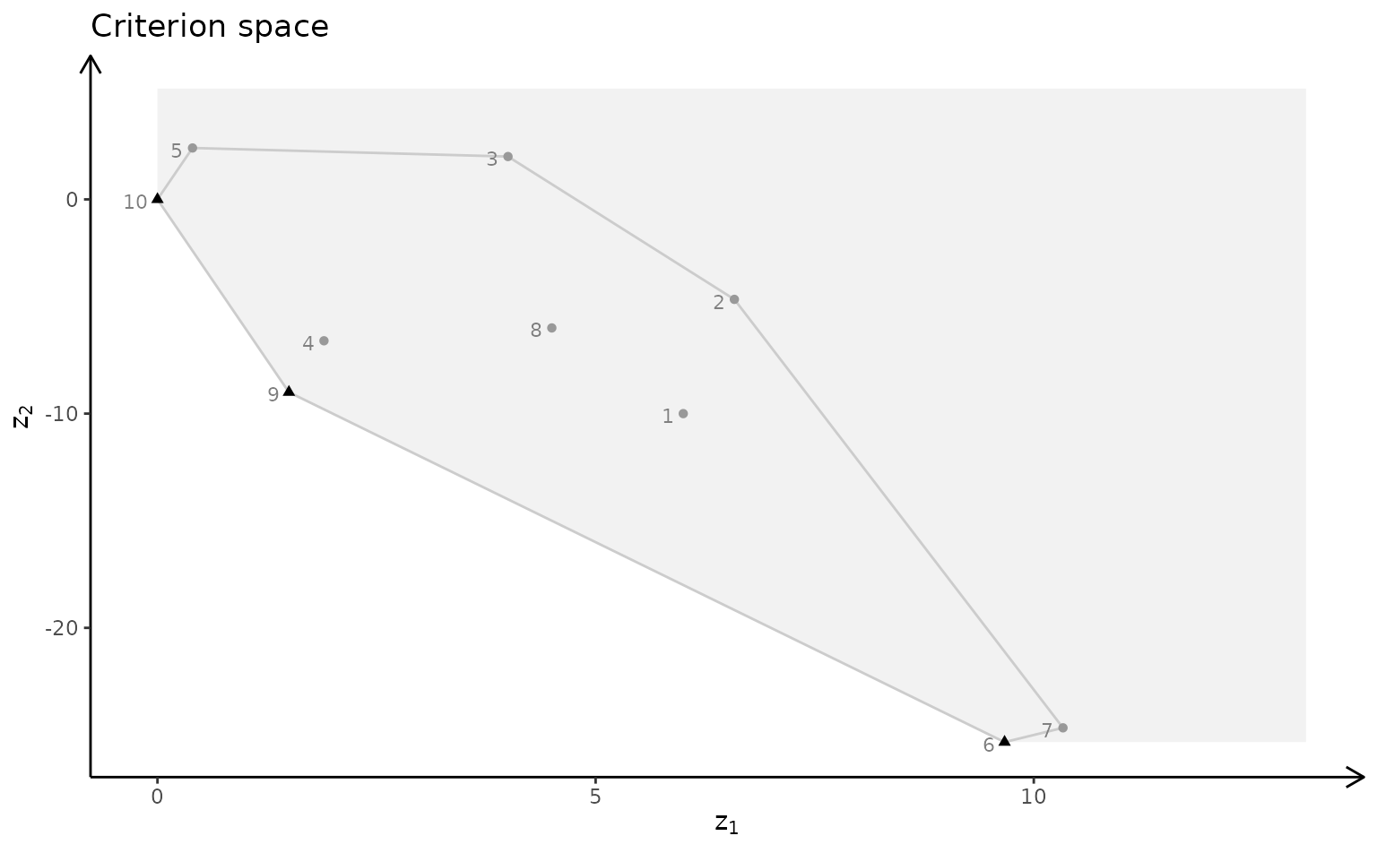
ILP model (solution space):
plotSol(A, b, type = c("i","i","i"))ILP model (criterion space):
plotCrit(A, b, obj, type = c("i","i","i"))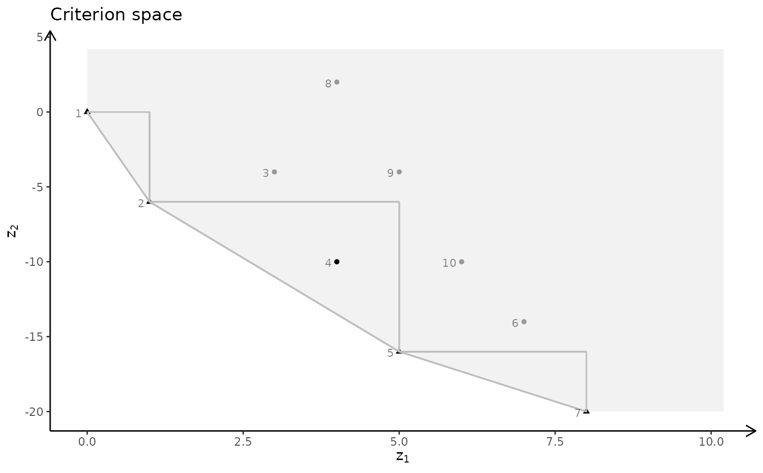
LaTeX support
You may create a TikZ file of the 2D plots for LaTeX using
library(tikzDevice)
tikz(file = "plot_polytope.tex", standAlone=F, width = 7, height = 6)
plotPolytope(
   A,
   b,
   obj,
   type = rep("i", ncol(A)),
   crit = "max",
   faces = rep("c", ncol(A)),
   plotFaces = TRUE,
   plotFeasible = TRUE,
   plotOptimum = TRUE,
   labels = "coord"
)
dev.off()
Further examples
For further examples see the documentation, the vignettes and the articles.
library(gMOIP)
browseVignettes('gMOIP')
example("gMOIP-package")