Plot the polytope (bounded convex set) of a linear mathematical program (Ax <= b)
Source:R/plot.R
plotPolytope.RdThis is a wrapper function calling plotPolytope2D() (2D graphics) and
plotPolytope3D() (3D graphics).
Arguments
- A
The constraint matrix.
- b
Right hand side.
- obj
A vector with objective coefficients.
- type
A character vector of same length as number of variables. If entry k is 'i' variable \(k\) must be integer and if 'c' continuous.
- nonneg
A boolean vector of same length as number of variables. If entry k is TRUE then variable k must be non-negative.
- crit
Either max or min (only used if add the iso-profit line)
- faces
A character vector of same length as number of variables. If entry k is 'i' variable \(k\) must be integer and if 'c' continuous. Useful if e.g. want to show the linear relaxation of an IP.
- plotFaces
If
Truethen plot the faces.- plotFeasible
If
Truethen plot the feasible points/segments (relevant for IPLP/MILP).- plotOptimum
Show the optimum corner solution point (if alternative solutions only one is shown) and add the iso-profit line.
- latex
If
Truemake latex math labels for TikZ.- labels
If
NULLdon't add any labels. If 'n' no labels but show the points. If equalcoordadd coordinates to the points. Otherwise number all points from one.- ...
If 2D, further arguments passed on the the
ggplotplotting functions. This must be done as lists. Currently the following arguments are supported:argsFaces: A list of arguments forplotHull2D.argsFeasible: A list of arguments forggplot2functions:geom_point: A list of arguments forggplot2::geom_point.geom_line: A list of arguments forggplot2::geom_line.
argsLabels: A list of arguments forggplot2functions:geom_text: A list of arguments forggplot2::geom_text.
argsOptimum:geom_point: A list of arguments forggplot2::geom_point.geom_abline: A list of arguments forggplot2::geom_abline.geom_label: A list of arguments forggplot2::geom_label.
argsTheme: A list of arguments forggplot2::theme.
If 3D further arguments passed on the the RGL plotting functions. This must be done as lists. Currently the following arguments are supported:
argsAxes3d: A list of arguments forrgl::axes3d.argsPlot3d: A list of arguments forrgl::plot3dto open the RGL window.argsTitle3d: A list of arguments forrgl::title3d.argsFaces: A list of arguments forplotHull3D.argsFeasible: A list of arguments for RGL functions:points3d: A list of arguments forrgl::points3d.segments3d: A list of arguments forrgl::segments3d.triangles3d: A list of arguments forrgl::triangles3d.
argsLabels: A list of arguments for RGL functions:points3d: A list of arguments forrgl::points3d.text3d: A list of arguments forrgl::text3d.
argsOptimum: A list of arguments for RGL functions:points3d: A list of arguments forrgl::points3d.
Note
The feasible region defined by the constraints must be bounded (i.e. no extreme rays) otherwise you may see strange results.
Author
Lars Relund lars@relund.dk
Examples
#### 2D examples ####
# Define the model max/min coeff*x st. Ax<=b, x>=0
A <- matrix(c(-3,2,2,4,9,10), ncol = 2, byrow = TRUE)
b <- c(3,27,90)
obj <- c(7.75, 10)
## LP model
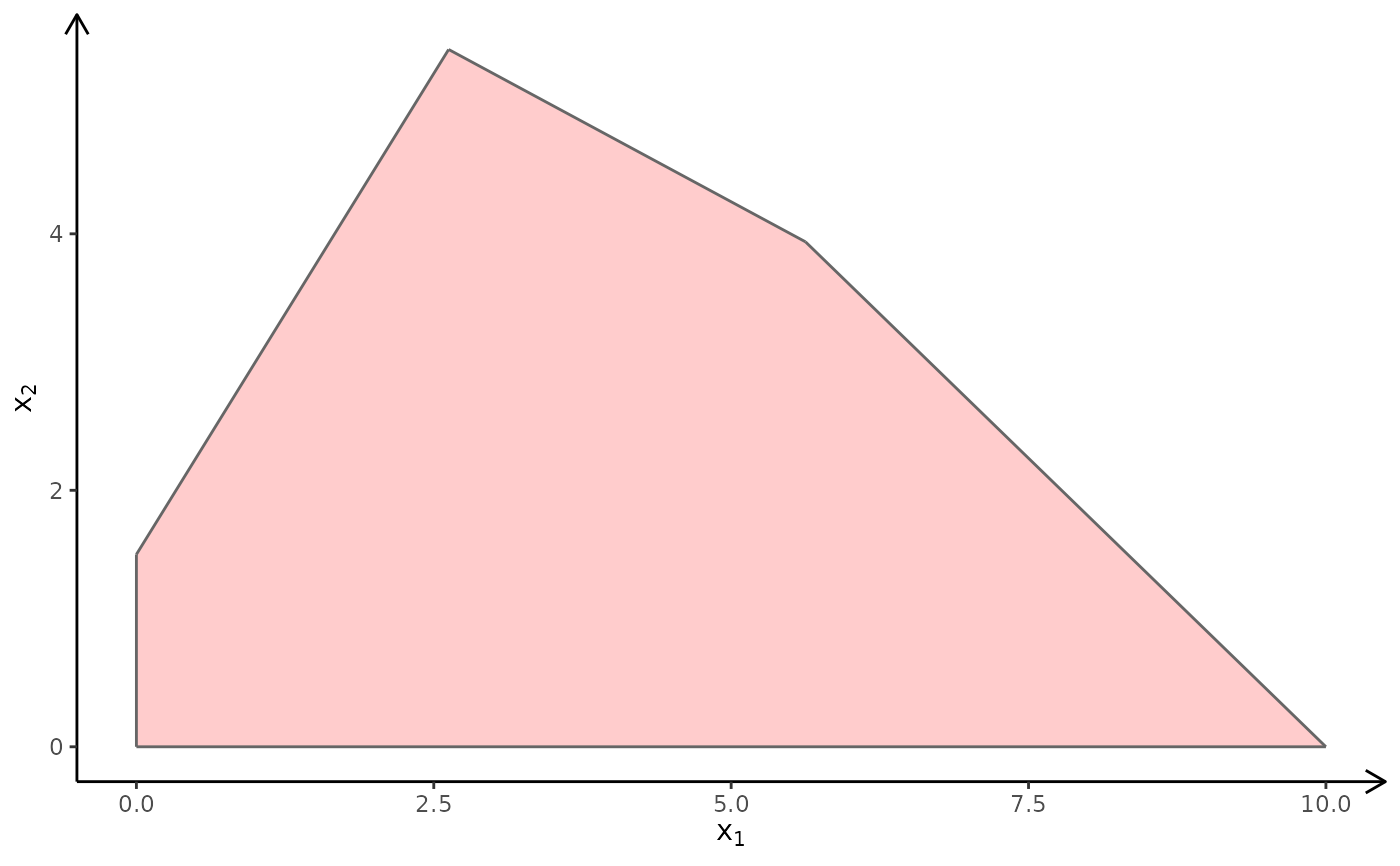
# The polytope with the corner points
plotPolytope(
A,
b,
obj,
type = rep("c", ncol(A)),
crit = "max",
faces = rep("c", ncol(A)),
plotFaces = TRUE,
plotFeasible = TRUE,
plotOptimum = FALSE,
labels = NULL,
argsFaces = list(argsGeom_polygon = list(fill = "red"))
)
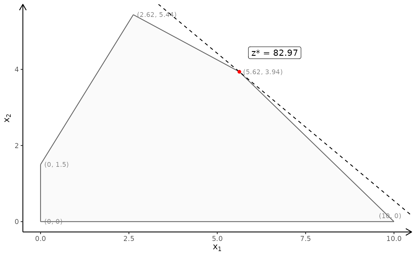
 # With optimum and labels:
plotPolytope(
A,
b,
obj,
type = rep("c", ncol(A)),
crit = "max",
faces = rep("c", ncol(A)),
plotFaces = TRUE,
plotFeasible = TRUE,
plotOptimum = TRUE,
labels = "coord",
argsOptimum = list(lty="solid")
)
# With optimum and labels:
plotPolytope(
A,
b,
obj,
type = rep("c", ncol(A)),
crit = "max",
faces = rep("c", ncol(A)),
plotFaces = TRUE,
plotFeasible = TRUE,
plotOptimum = TRUE,
labels = "coord",
argsOptimum = list(lty="solid")
)
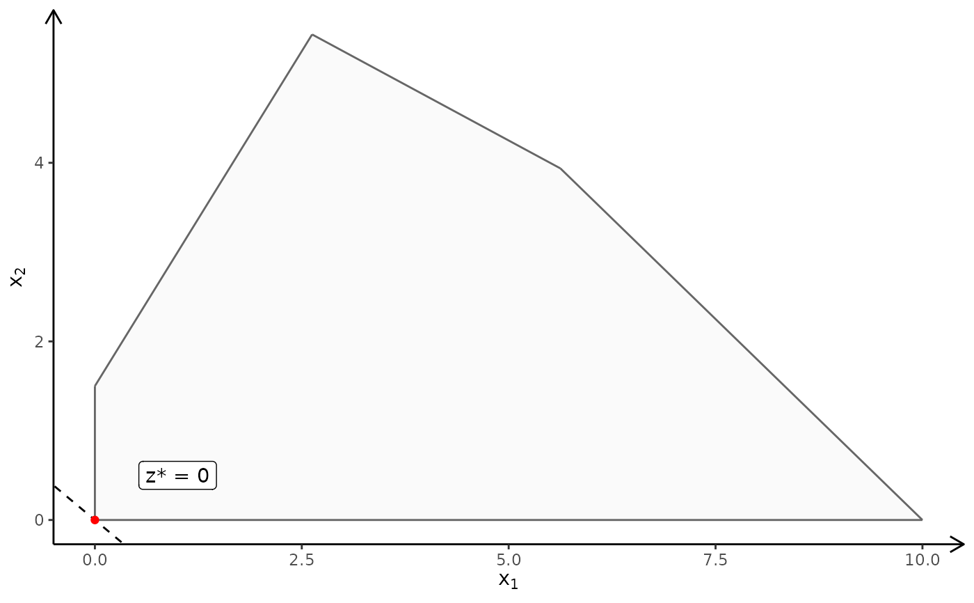
 # Minimize:
plotPolytope(
A,
b,
obj,
type = rep("c", ncol(A)),
crit = "min",
faces = rep("c", ncol(A)),
plotFaces = TRUE,
plotFeasible = TRUE,
plotOptimum = TRUE,
labels = "n"
)
# Minimize:
plotPolytope(
A,
b,
obj,
type = rep("c", ncol(A)),
crit = "min",
faces = rep("c", ncol(A)),
plotFaces = TRUE,
plotFeasible = TRUE,
plotOptimum = TRUE,
labels = "n"
)
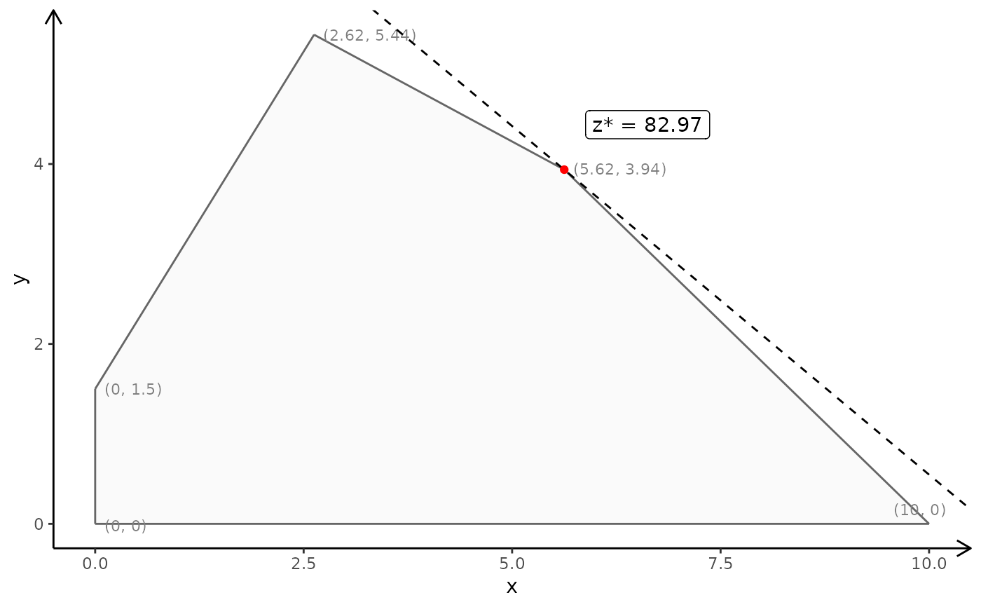
 # Note return a ggplot so can e.g. add other labels on e.g. the axes:
p <- plotPolytope(
A,
b,
obj,
type = rep("c", ncol(A)),
crit = "max",
faces = rep("c", ncol(A)),
plotFaces = TRUE,
plotFeasible = TRUE,
plotOptimum = TRUE,
labels = "coord"
)
p + ggplot2::xlab("x") + ggplot2::ylab("y")
# Note return a ggplot so can e.g. add other labels on e.g. the axes:
p <- plotPolytope(
A,
b,
obj,
type = rep("c", ncol(A)),
crit = "max",
faces = rep("c", ncol(A)),
plotFaces = TRUE,
plotFeasible = TRUE,
plotOptimum = TRUE,
labels = "coord"
)
p + ggplot2::xlab("x") + ggplot2::ylab("y")
 # More examples
# \donttest{
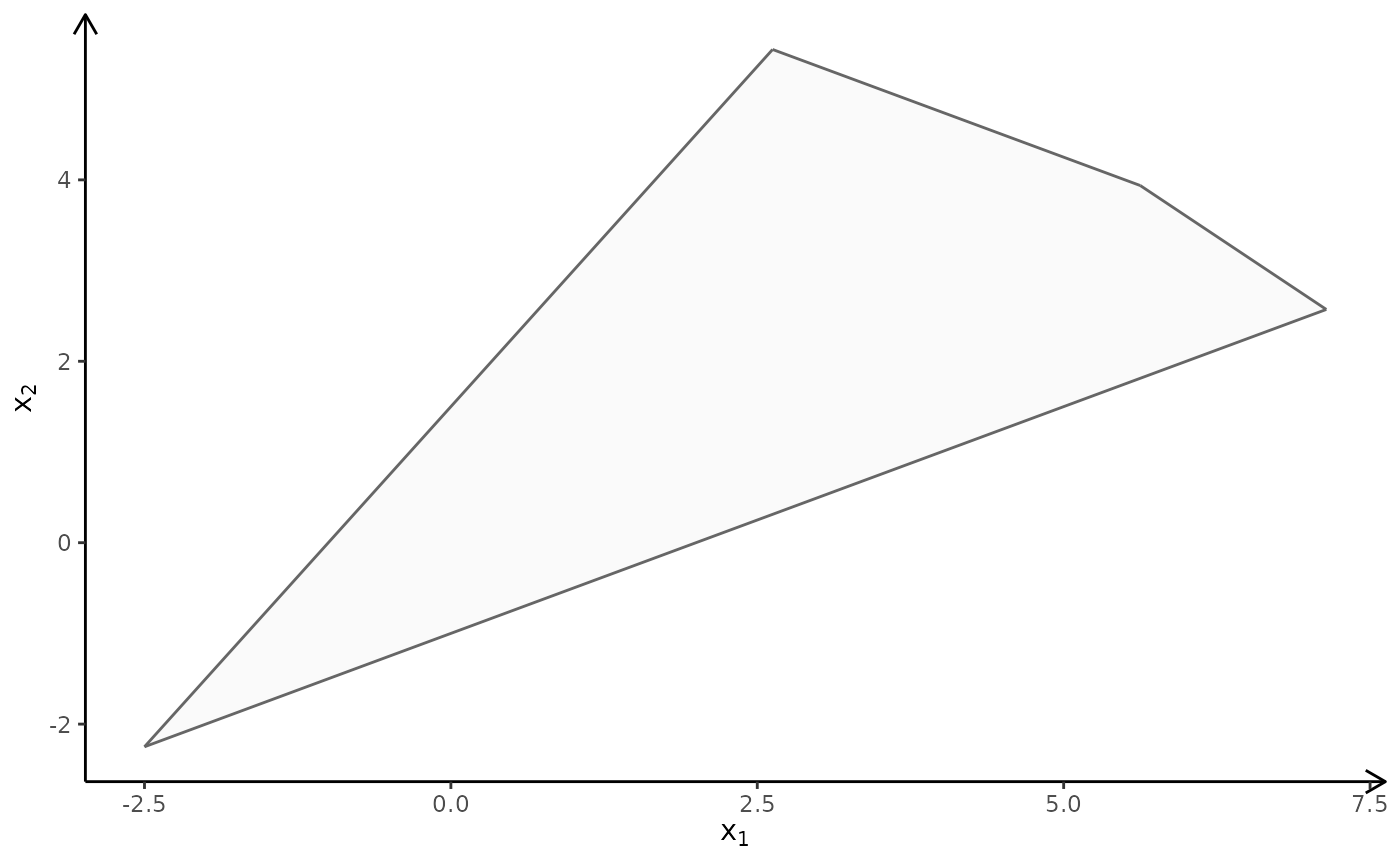
## LP-model with no non-negativity constraints
A <- matrix(c(-3, 2, 2, 4, 9, 10, 1, -2), ncol = 2, byrow = TRUE)
b <- c(3, 27, 90, 2)
obj <- c(7.75, 10)
plotPolytope(
A,
b,
obj,
type = rep("c", ncol(A)),
nonneg = rep(FALSE, ncol(A)),
crit = "max",
faces = rep("c", ncol(A)),
plotFaces = TRUE,
plotFeasible = TRUE,
plotOptimum = FALSE,
labels = NULL
)
# More examples
# \donttest{
## LP-model with no non-negativity constraints
A <- matrix(c(-3, 2, 2, 4, 9, 10, 1, -2), ncol = 2, byrow = TRUE)
b <- c(3, 27, 90, 2)
obj <- c(7.75, 10)
plotPolytope(
A,
b,
obj,
type = rep("c", ncol(A)),
nonneg = rep(FALSE, ncol(A)),
crit = "max",
faces = rep("c", ncol(A)),
plotFaces = TRUE,
plotFeasible = TRUE,
plotOptimum = FALSE,
labels = NULL
)
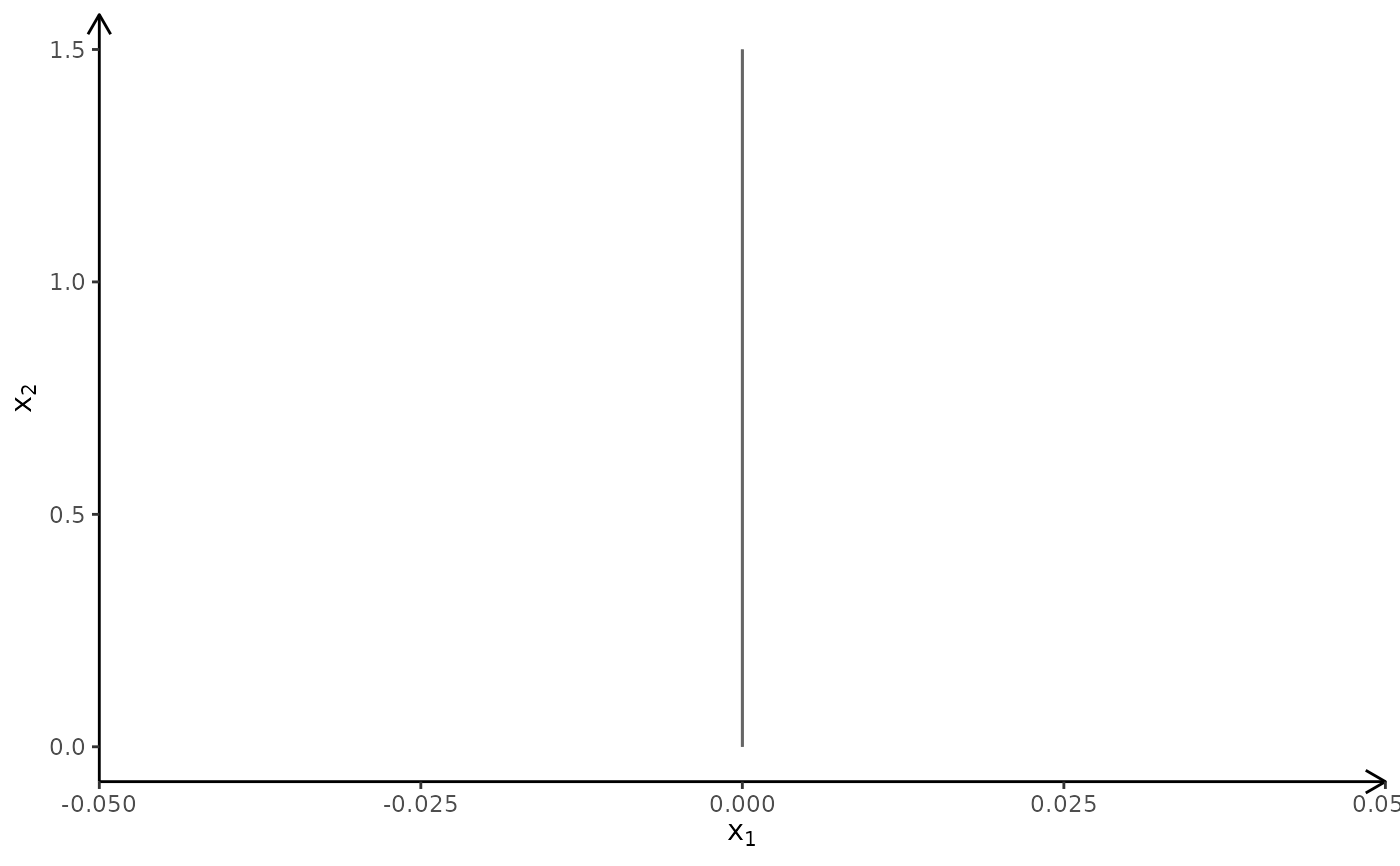
 ## The package don't plot feasible regions that are unbounded e.g if we drop the 2 and 3 constraint
A <- matrix(c(-3,2), ncol = 2, byrow = TRUE)
b <- c(3)
obj <- c(7.75, 10)
# Wrong plot
plotPolytope(
A,
b,
obj,
type = rep("c", ncol(A)),
crit = "max",
faces = rep("c", ncol(A)),
plotFaces = TRUE,
plotFeasible = TRUE,
plotOptimum = FALSE,
labels = NULL
)
## The package don't plot feasible regions that are unbounded e.g if we drop the 2 and 3 constraint
A <- matrix(c(-3,2), ncol = 2, byrow = TRUE)
b <- c(3)
obj <- c(7.75, 10)
# Wrong plot
plotPolytope(
A,
b,
obj,
type = rep("c", ncol(A)),
crit = "max",
faces = rep("c", ncol(A)),
plotFaces = TRUE,
plotFeasible = TRUE,
plotOptimum = FALSE,
labels = NULL
)
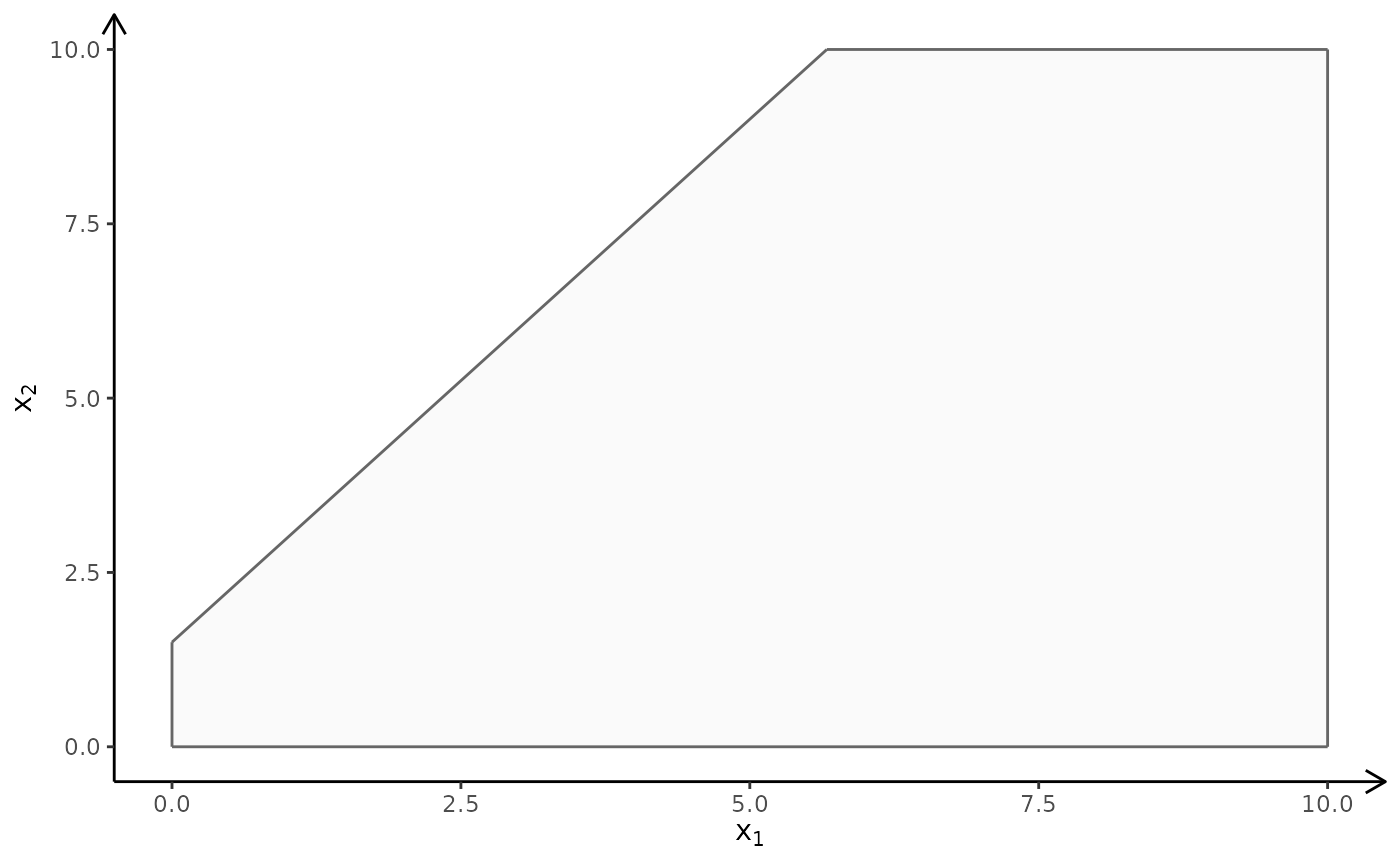
 # One solution is to add a bounding box and check if the bounding box is binding
A <- rbind(A, c(1,0), c(0,1))
b <- c(b, 10, 10)
plotPolytope(
A,
b,
obj,
type = rep("c", ncol(A)),
crit = "max",
faces = rep("c", ncol(A)),
plotFaces = TRUE,
plotFeasible = TRUE,
plotOptimum = FALSE,
labels = NULL
)
# One solution is to add a bounding box and check if the bounding box is binding
A <- rbind(A, c(1,0), c(0,1))
b <- c(b, 10, 10)
plotPolytope(
A,
b,
obj,
type = rep("c", ncol(A)),
crit = "max",
faces = rep("c", ncol(A)),
plotFaces = TRUE,
plotFeasible = TRUE,
plotOptimum = FALSE,
labels = NULL
)
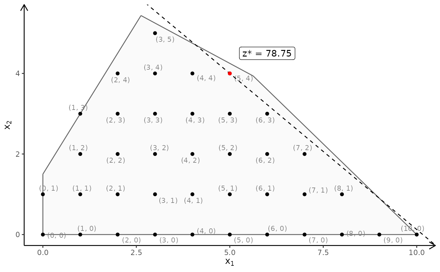
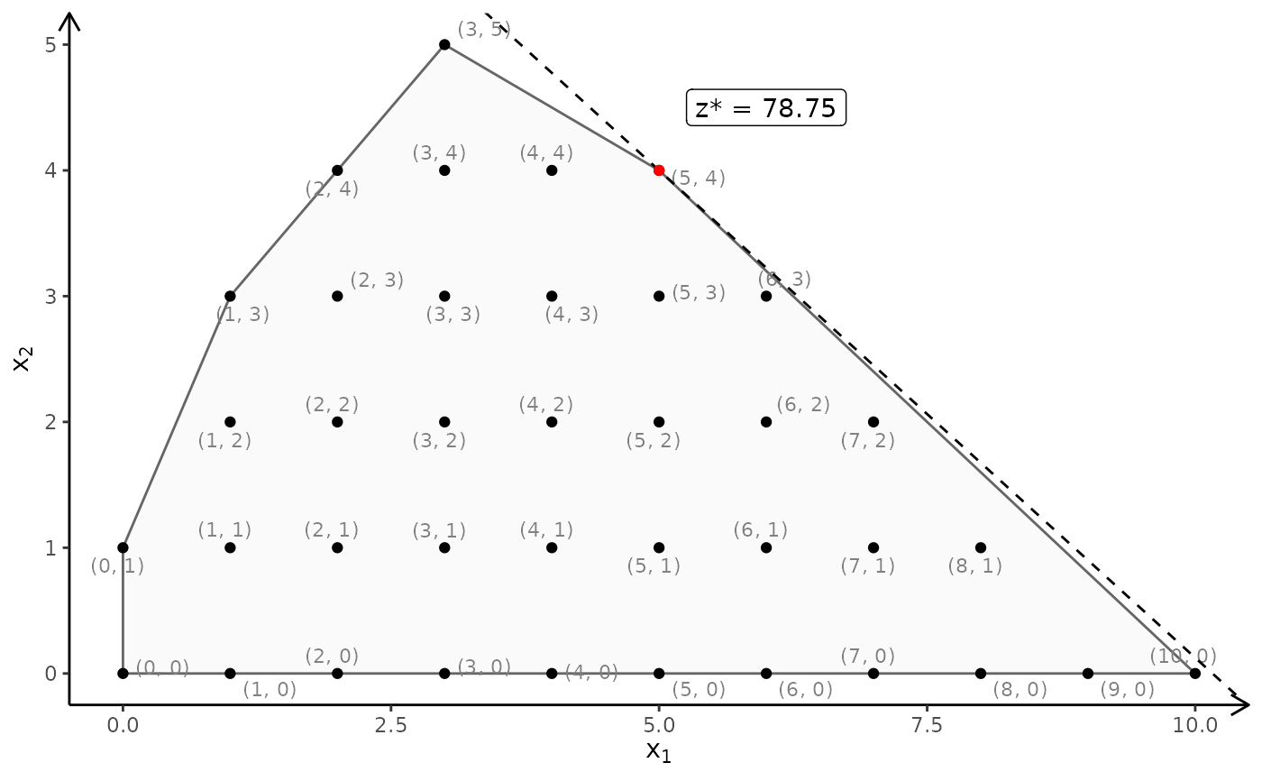
 ## ILP model
A <- matrix(c(-3,2,2,4,9,10), ncol = 2, byrow = TRUE)
b <- c(3,27,90)
obj <- c(7.75, 10)
# ILP model with LP faces:
plotPolytope(
A,
b,
obj,
type = rep("i", ncol(A)),
crit = "max",
faces = rep("c", ncol(A)),
plotFaces = TRUE,
plotFeasible = TRUE,
plotOptimum = TRUE,
labels = "coord",
argsLabels = list(size = 4, color = "blue"),
argsFeasible = list(color = "red", size = 3)
)
## ILP model
A <- matrix(c(-3,2,2,4,9,10), ncol = 2, byrow = TRUE)
b <- c(3,27,90)
obj <- c(7.75, 10)
# ILP model with LP faces:
plotPolytope(
A,
b,
obj,
type = rep("i", ncol(A)),
crit = "max",
faces = rep("c", ncol(A)),
plotFaces = TRUE,
plotFeasible = TRUE,
plotOptimum = TRUE,
labels = "coord",
argsLabels = list(size = 4, color = "blue"),
argsFeasible = list(color = "red", size = 3)
)
 #ILP model with IP faces:
plotPolytope(
A,
b,
obj,
type = rep("i", ncol(A)),
crit = "max",
faces = rep("i", ncol(A)),
plotFaces = TRUE,
plotFeasible = TRUE,
plotOptimum = TRUE,
labels = "coord"
)
#ILP model with IP faces:
plotPolytope(
A,
b,
obj,
type = rep("i", ncol(A)),
crit = "max",
faces = rep("i", ncol(A)),
plotFaces = TRUE,
plotFeasible = TRUE,
plotOptimum = TRUE,
labels = "coord"
)
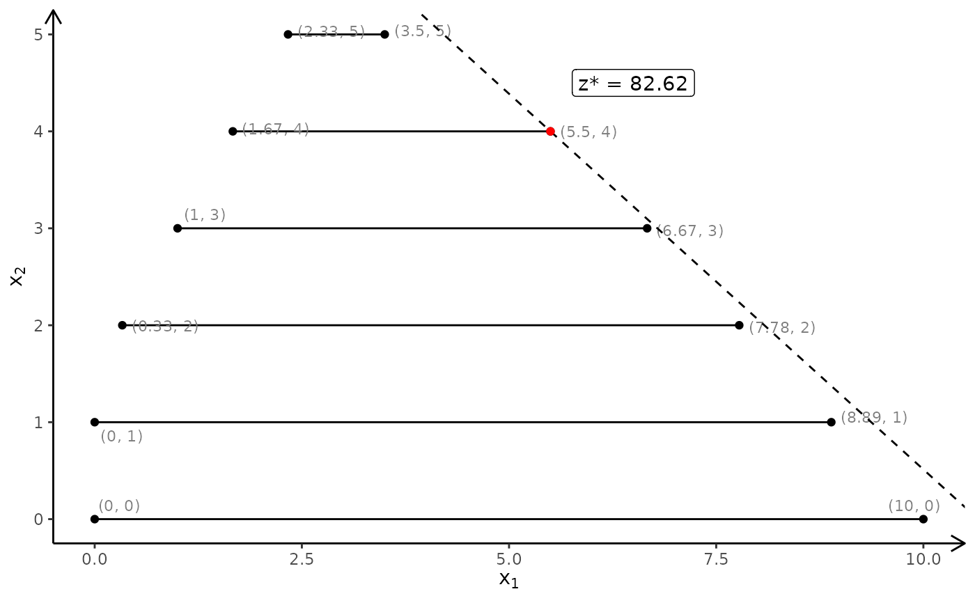
 ## MILP model
A <- matrix(c(-3,2,2,4,9,10), ncol = 2, byrow = TRUE)
b <- c(3,27,90)
obj <- c(7.75, 10)
# Second coordinate integer
plotPolytope(
A,
b,
obj,
type = c("c", "i"),
crit = "max",
faces = c("c", "i"),
plotFaces = FALSE,
plotFeasible = TRUE,
plotOptimum = TRUE,
labels = "coord",
argsFeasible = list(color = "red")
)
## MILP model
A <- matrix(c(-3,2,2,4,9,10), ncol = 2, byrow = TRUE)
b <- c(3,27,90)
obj <- c(7.75, 10)
# Second coordinate integer
plotPolytope(
A,
b,
obj,
type = c("c", "i"),
crit = "max",
faces = c("c", "i"),
plotFaces = FALSE,
plotFeasible = TRUE,
plotOptimum = TRUE,
labels = "coord",
argsFeasible = list(color = "red")
)
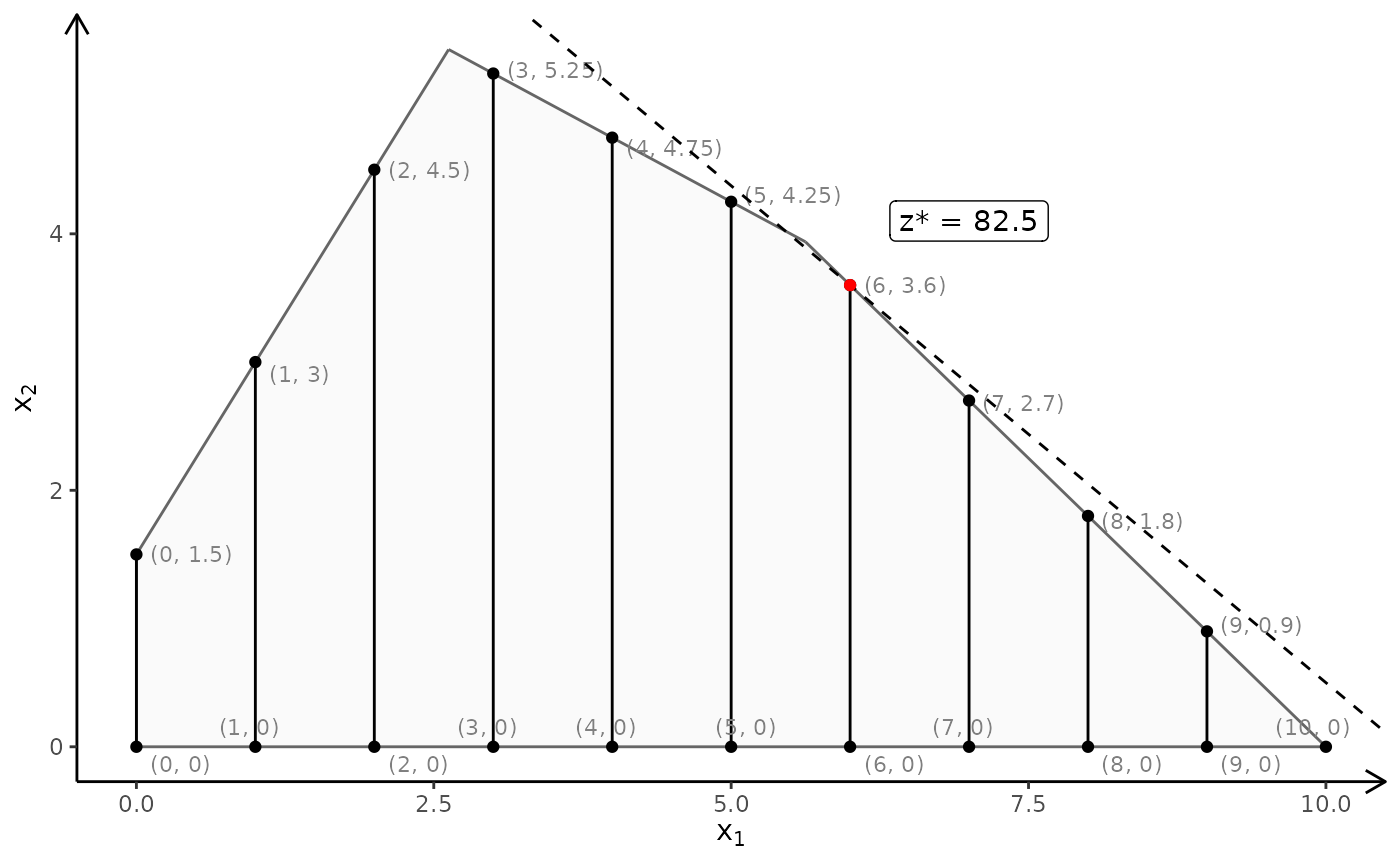
 # First coordinate integer and with LP faces:
plotPolytope(
A,
b,
obj,
type = c("i", "c"),
crit = "max",
faces = c("c", "c"),
plotFaces = TRUE,
plotFeasible = TRUE,
plotOptimum = TRUE,
labels = "coord"
)
# First coordinate integer and with LP faces:
plotPolytope(
A,
b,
obj,
type = c("i", "c"),
crit = "max",
faces = c("c", "c"),
plotFaces = TRUE,
plotFeasible = TRUE,
plotOptimum = TRUE,
labels = "coord"
)
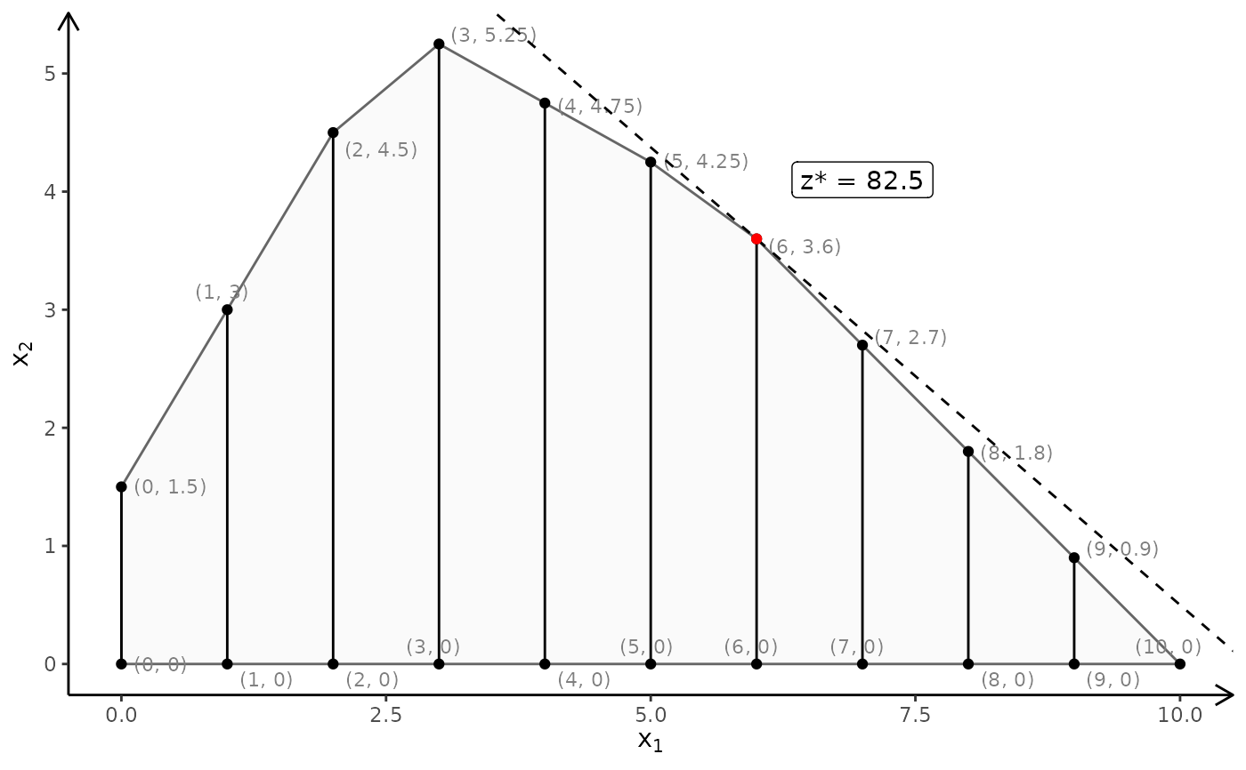
 # First coordinate integer and with LP faces:
plotPolytope(
A,
b,
obj,
type = c("i", "c"),
crit = "max",
faces = c("i", "c"),
plotFaces = TRUE,
plotFeasible = TRUE,
plotOptimum = TRUE,
labels = "coord"
)
# First coordinate integer and with LP faces:
plotPolytope(
A,
b,
obj,
type = c("i", "c"),
crit = "max",
faces = c("i", "c"),
plotFaces = TRUE,
plotFeasible = TRUE,
plotOptimum = TRUE,
labels = "coord"
)
 # }
#### 3D examples ####
# \donttest{
# Ex 1
view <- matrix( c(-0.412063330411911, -0.228006735444069, 0.882166087627411, 0, 0.910147845745087,
-0.0574885793030262, 0.410274744033813, 0, -0.042830865830183, 0.97196090221405,
0.231208890676498, 0, 0, 0, 0, 1), nc = 4)
loadView(v = view)
# }
#### 3D examples ####
# \donttest{
# Ex 1
view <- matrix( c(-0.412063330411911, -0.228006735444069, 0.882166087627411, 0, 0.910147845745087,
-0.0574885793030262, 0.410274744033813, 0, -0.042830865830183, 0.97196090221405,
0.231208890676498, 0, 0, 0, 0, 1), nc = 4)
loadView(v = view)
3D plot
A <- matrix( c(
3, 2, 5,
2, 1, 1,
1, 1, 3,
5, 2, 4
), nc = 3, byrow = TRUE)
b <- c(55, 26, 30, 57)
obj <- c(20, 10, 15)
# LP model
plotPolytope(A, b, plotOptimum = TRUE, obj = obj, labels = "coord")
#> Warning: edge not found:1 2
3D plot
plotPolytope(A, b, plotOptimum = TRUE, obj = obj, labels = "coord",
argsFaces = list(drawLines = FALSE, argsPolygon3d = list(alpha = 0.95)),
argsLabels = list(points3d = list(color = "blue")))
#> Warning: edge not found:1 2
3D plot
# ILP model
plotPolytope(A, b, faces = c("c","c","c"), type = c("i","i","i"), plotOptimum = TRUE, obj = obj)
#> Warning: edge not found:1 2
3D plot
# MILP model
plotPolytope(A, b, faces = c("c","c","c"), type = c("i","c","i"), plotOptimum = TRUE, obj = obj)
#> Warning: edge not found:1 2
3D plot
plotPolytope(A, b, faces = c("c","c","c"), type = c("c","i","i"), plotOptimum = TRUE, obj = obj)
#> Warning: edge not found:1 2
3D plot
plotPolytope(A, b, faces = c("c","c","c"), type = c("i","i","c"), plotOptimum = TRUE, obj = obj)
#> Warning: edge not found:1 2
3D plot
plotPolytope(A, b, faces = c("c","c","c"), type = c("i","i","c"), plotFaces = FALSE)
3D plot
plotPolytope(A, b, type = c("i","c","c"), plotOptimum = TRUE, obj = obj, plotFaces = FALSE)
3D plot
plotPolytope(A, b, type = c("c","i","c"), plotOptimum = TRUE, obj = obj, plotFaces = FALSE)
3D plot
plotPolytope(A, b, type = c("c","c","i"), plotOptimum = TRUE, obj = obj, plotFaces = FALSE)
# Ex 2
view <- matrix( c(-0.812462985515594, -0.029454167932272, 0.582268416881561, 0, 0.579295456409454,
-0.153386667370796, 0.800555109977722, 0, 0.0657325685024261, 0.987727105617523,
0.14168381690979, 0, 0, 0, 0, 1), nc = 4)
loadView(v = view)
3D plot
A <- matrix( c(
1, 1, 1,
3, 0, 1
), nc = 3, byrow = TRUE)
b <- c(10, 24)
obj <- c(20, 10, 15)
plotPolytope(A, b, plotOptimum = TRUE, obj = obj, labels = "coord")
3D plot
# ILP model
plotPolytope(A, b, faces = c("c","c","c"), type = c("i","i","i"), plotOptimum = TRUE, obj = obj)
3D plot
# MILP model
plotPolytope(A, b, faces = c("c","c","c"), type = c("i","c","i"), plotOptimum = TRUE, obj = obj)
3D plot
plotPolytope(A, b, faces = c("c","c","c"), type = c("c","i","i"), plotOptimum = TRUE, obj = obj)
3D plot
plotPolytope(A, b, faces = c("c","c","c"), type = c("i","i","c"), plotOptimum = TRUE, obj = obj)
3D plot
plotPolytope(A, b, faces = c("c","c","c"), type = c("i","i","c"), plotFaces = FALSE)
3D plot
plotPolytope(A, b, type = c("i","c","c"), plotOptimum = TRUE, obj = obj, plotFaces = FALSE)
3D plot
plotPolytope(A, b, type = c("c","i","c"), plotOptimum = TRUE, obj = obj, plotFaces = FALSE)
3D plot
plotPolytope(A, b, type = c("c","c","i"), plotOptimum = TRUE, obj = obj, plotFaces = FALSE)
# Ex 3
view <- matrix( c(0.976349174976349, -0.202332556247711, 0.0761845782399178, 0, 0.0903248339891434,
0.701892614364624, 0.706531345844269, 0, -0.196427255868912, -0.682940244674683,
0.703568696975708, 0, 0, 0, 0, 1), nc = 4)
loadView(v = view)
3D plot
A <- matrix( c(
-1, 1, 0,
1, 4, 0,
2, 1, 0,
3, -4, 0,
0, 0, 4
), nc = 3, byrow = TRUE)
b <- c(5, 45, 27, 24, 10)
obj <- c(5, 45, 15)
plotPolytope(A, b, plotOptimum = TRUE, obj = obj, labels = "coord")
3D plot
# ILP model
plotPolytope(A, b, faces = c("c","c","c"), type = c("i","i","i"), plotOptimum = TRUE, obj = obj)
3D plot
# MILP model
plotPolytope(A, b, faces = c("c","c","c"), type = c("i","c","i"), plotOptimum = TRUE, obj = obj)
3D plot
plotPolytope(A, b, faces = c("c","c","c"), type = c("c","i","i"), plotOptimum = TRUE, obj = obj)
3D plot
plotPolytope(A, b, faces = c("c","c","c"), type = c("i","i","c"), plotOptimum = TRUE, obj = obj)
3D plot
plotPolytope(A, b, faces = c("c","c","c"), type = c("i","i","c"), plotFaces = FALSE)
3D plot
plotPolytope(A, b, type = c("i","c","c"), plotOptimum = TRUE, obj = obj, plotFaces = FALSE)
3D plot
plotPolytope(A, b, type = c("c","i","c"), plotOptimum = TRUE, obj = obj, plotFaces = FALSE)
3D plot
plotPolytope(A, b, type = c("c","c","i"), plotOptimum = TRUE, obj = obj, plotFaces = FALSE)
# Ex 4
view <- matrix( c(-0.452365815639496, -0.446501553058624, 0.77201122045517, 0, 0.886364221572876,
-0.320795893669128, 0.333835482597351, 0, 0.0986008867621422, 0.835299551486969,
0.540881276130676, 0, 0, 0, 0, 1), nc = 4)
loadView(v = view)
3D plot
Ab <- matrix( c(
1, 1, 2, 5,
2, -1, 0, 3,
-1, 2, 1, 3,
0, -3, 5, 2
# 0, 1, 0, 4,
# 1, 0, 0, 4
), nc = 4, byrow = TRUE)
A <- Ab[,1:3]
b <- Ab[,4]
obj = c(1,1,3)
plotPolytope(A, b, plotOptimum = TRUE, obj = obj, labels = "coord")
3D plot
# ILP model
plotPolytope(A, b, faces = c("c","c","c"), type = c("i","i","i"), plotOptimum = TRUE, obj = obj)
3D plot
# MILP model
plotPolytope(A, b, faces = c("c","c","c"), type = c("i","c","i"), plotOptimum = TRUE, obj = obj)
3D plot
plotPolytope(A, b, faces = c("c","c","c"), type = c("c","i","i"), plotOptimum = TRUE, obj = obj)
3D plot
plotPolytope(A, b, faces = c("c","c","c"), type = c("i","i","c"), plotOptimum = TRUE, obj = obj)
3D plot
plotPolytope(A, b, faces = c("c","c","c"), type = c("i","i","c"), plotFaces = FALSE)
3D plot
plotPolytope(A, b, type = c("i","c","c"), plotOptimum = TRUE, obj = obj, plotFaces = FALSE)
3D plot
plotPolytope(A, b, type = c("c","i","c"), plotOptimum = TRUE, obj = obj, plotFaces = FALSE)
3D plot
plotPolytope(A, b, faces = c("c","c","c"), type = c("c","c","i"), plotOptimum = TRUE, obj = obj)
3D plot
# }