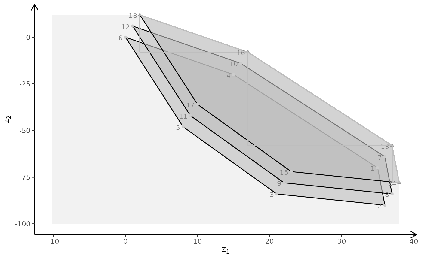
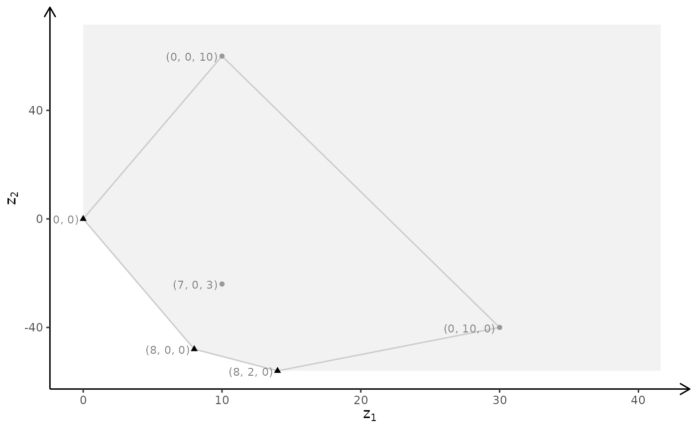
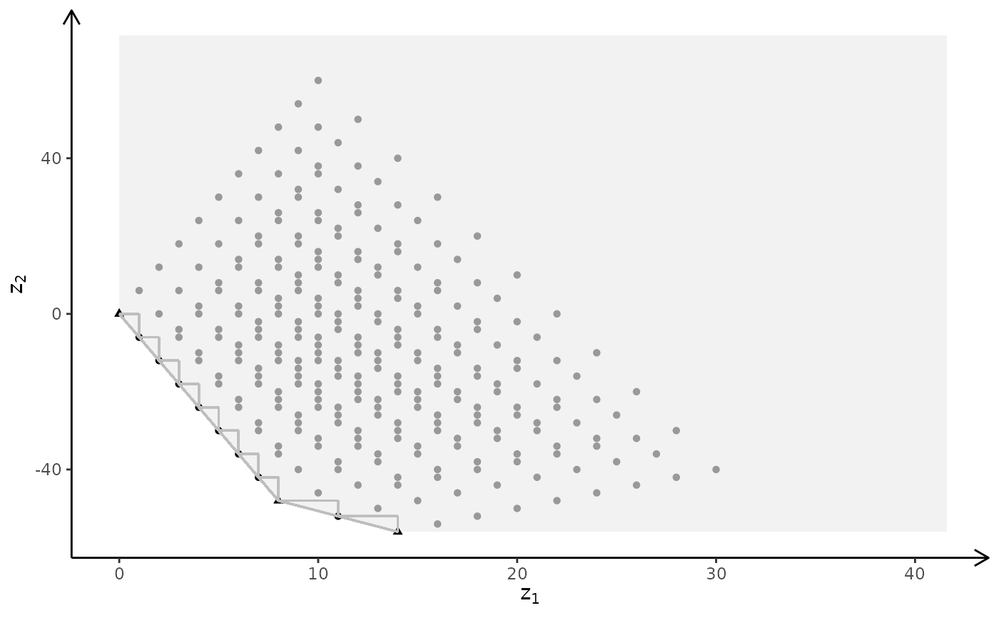
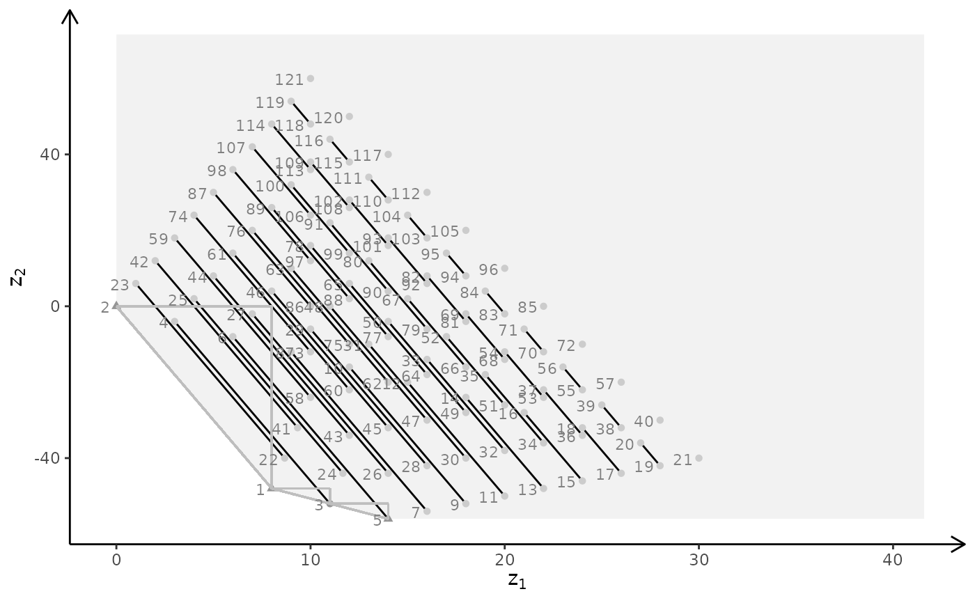
Create a plot of the criterion space of a bi-objective problem
Arguments
- A
The constraint matrix.
- b
Right hand side.
- obj
A p x n matrix(one row for each criterion).
- type
A character vector of same length as number of variables. If entry k is 'i' variable \(k\) must be integer and if 'c' continuous.
- nonneg
A boolean vector of same length as number of variables. If entry k is TRUE then variable k must be non-negative.
- crit
Either max or min (only used if add the iso-profit line).
- addTriangles
Add search triangles defined by the non-dominated extreme points.
- addHull
Add the convex hull and the rays.
- plotFeasible
If
Truethen plot the criterion points/slices.- latex
If true make latex math labels for TikZ.
- labels
If
NULLdon't add any labels. If 'n' no labels but show the points. If equalcoordadd coordinates to the points. Otherwise number all points from one.
Note
Currently only points are checked for dominance. That is, for MILP models some nondominated points may in fact be dominated by a segment.
Author
Lars Relund lars@relund.dk
Examples
### Set up 2D plot
# Function for plotting the solution and criterion space in one plot (two variables)
plotBiObj2D <- function(A, b, obj,
type = rep("c", ncol(A)),
crit = "max",
faces = rep("c", ncol(A)),
plotFaces = TRUE,
plotFeasible = TRUE,
plotOptimum = FALSE,
labels = "numb",
addTriangles = TRUE,
addHull = TRUE)
{
p1 <- plotPolytope(A, b, type = type, crit = crit, faces = faces, plotFaces = plotFaces,
plotFeasible = plotFeasible, plotOptimum = plotOptimum, labels = labels)
p2 <- plotCriterion2D(A, b, obj, type = type, crit = crit, addTriangles = addTriangles,
addHull = addHull, plotFeasible = plotFeasible, labels = labels)
gridExtra::grid.arrange(p1, p2, nrow = 1)
}
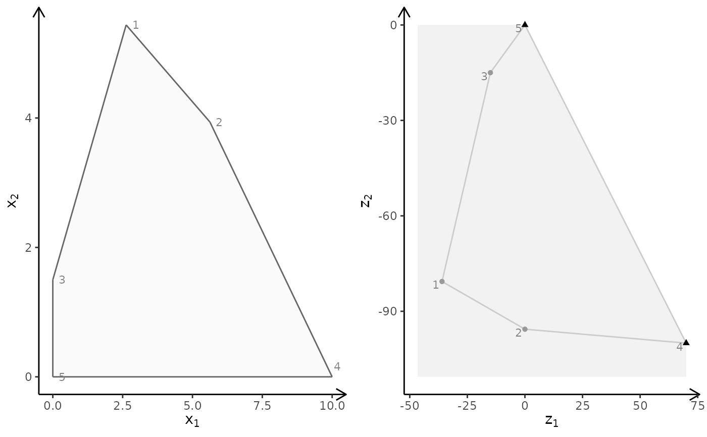
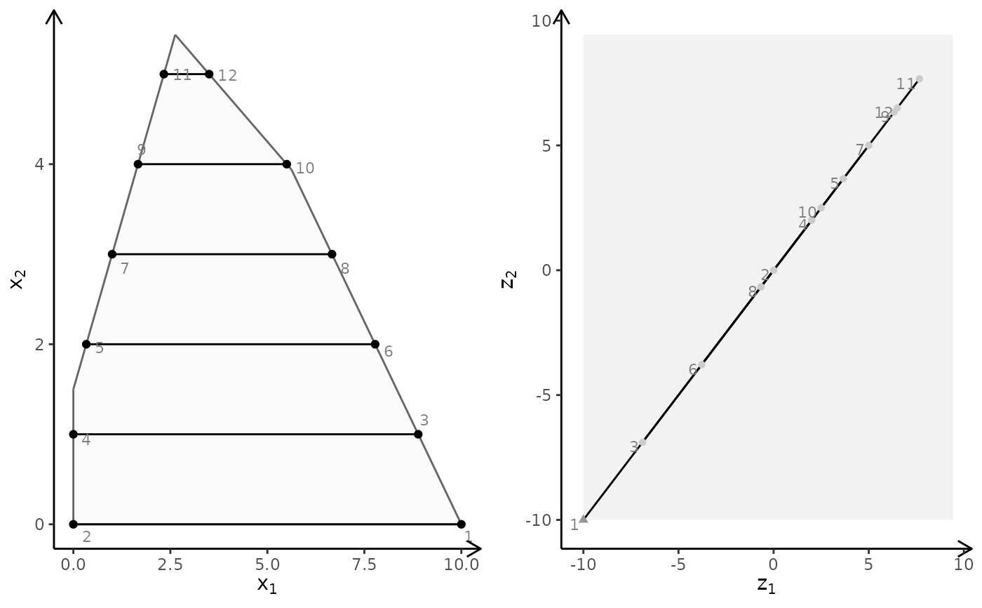
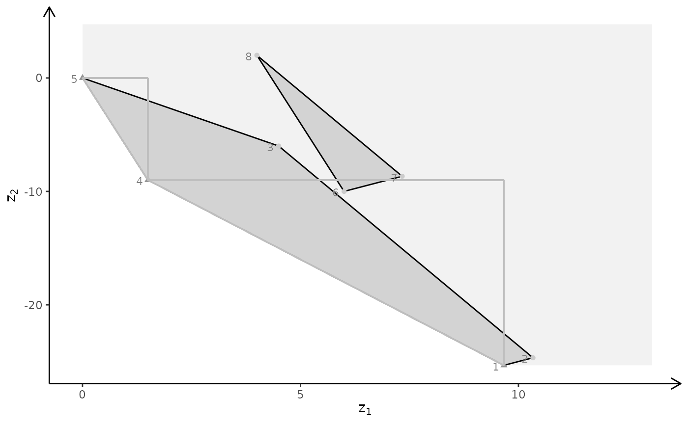
### Bi-objective problem with two variables
A <- matrix(c(-3,2,2,4,9,10), ncol = 2, byrow = TRUE)
b <- c(3,27,90)
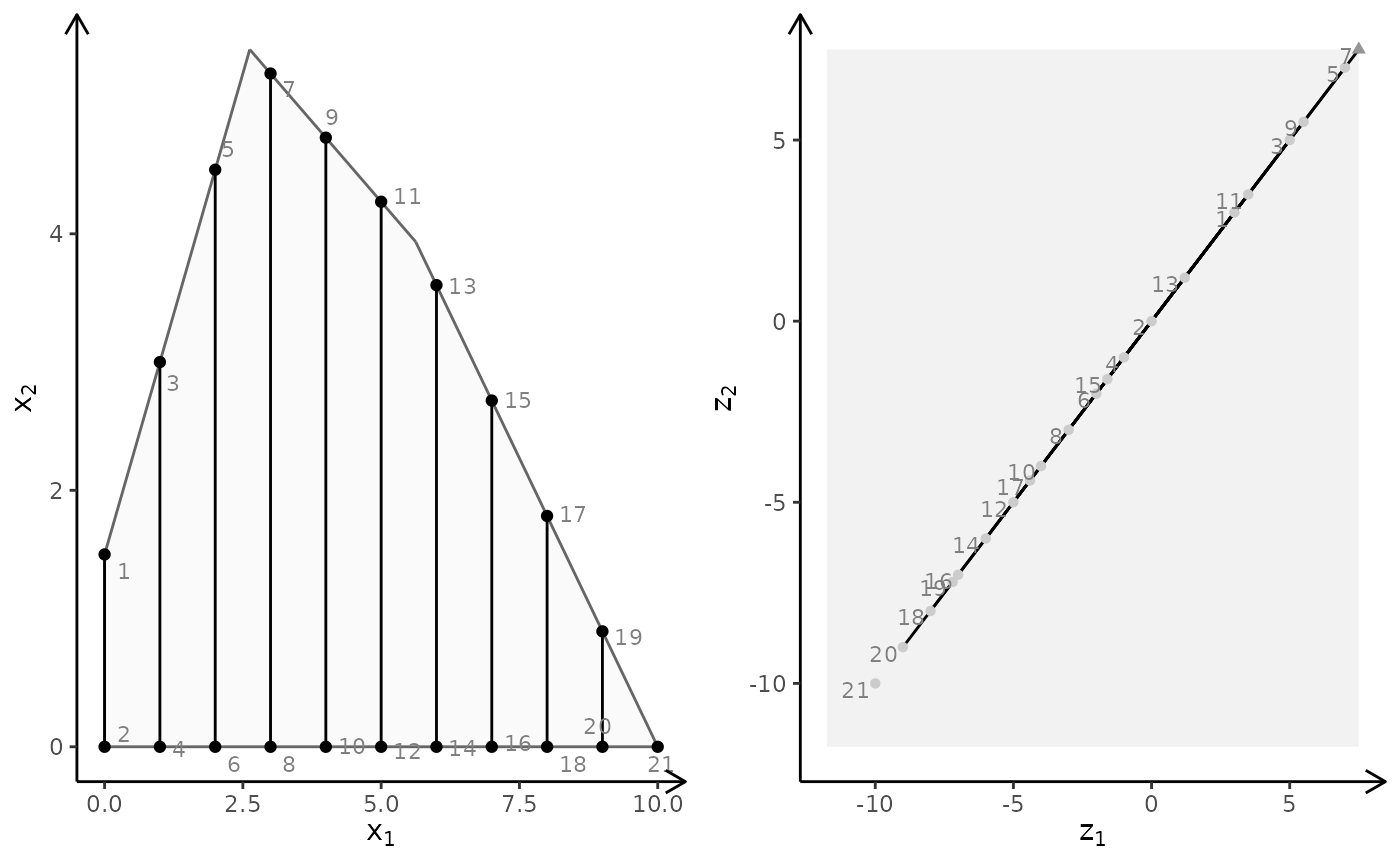
## LP model
obj <- matrix(
c(7, -10, # first criterion
-10, -10), # second criterion
nrow = 2)
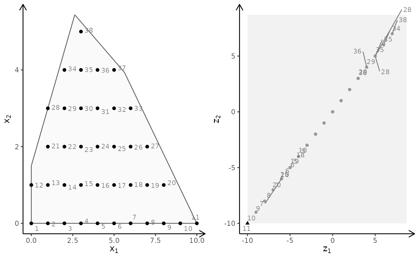
plotBiObj2D(A, b, obj, addTriangles = FALSE)
#> Warning: `aes_()` was deprecated in ggplot2 3.0.0.
#> ℹ Please use tidy evaluation idioms with `aes()`
#> ℹ The deprecated feature was likely used in the gMOIP package.
#> Please report the issue at <https://github.com/relund/gMOIP/issues>.
 # \donttest{
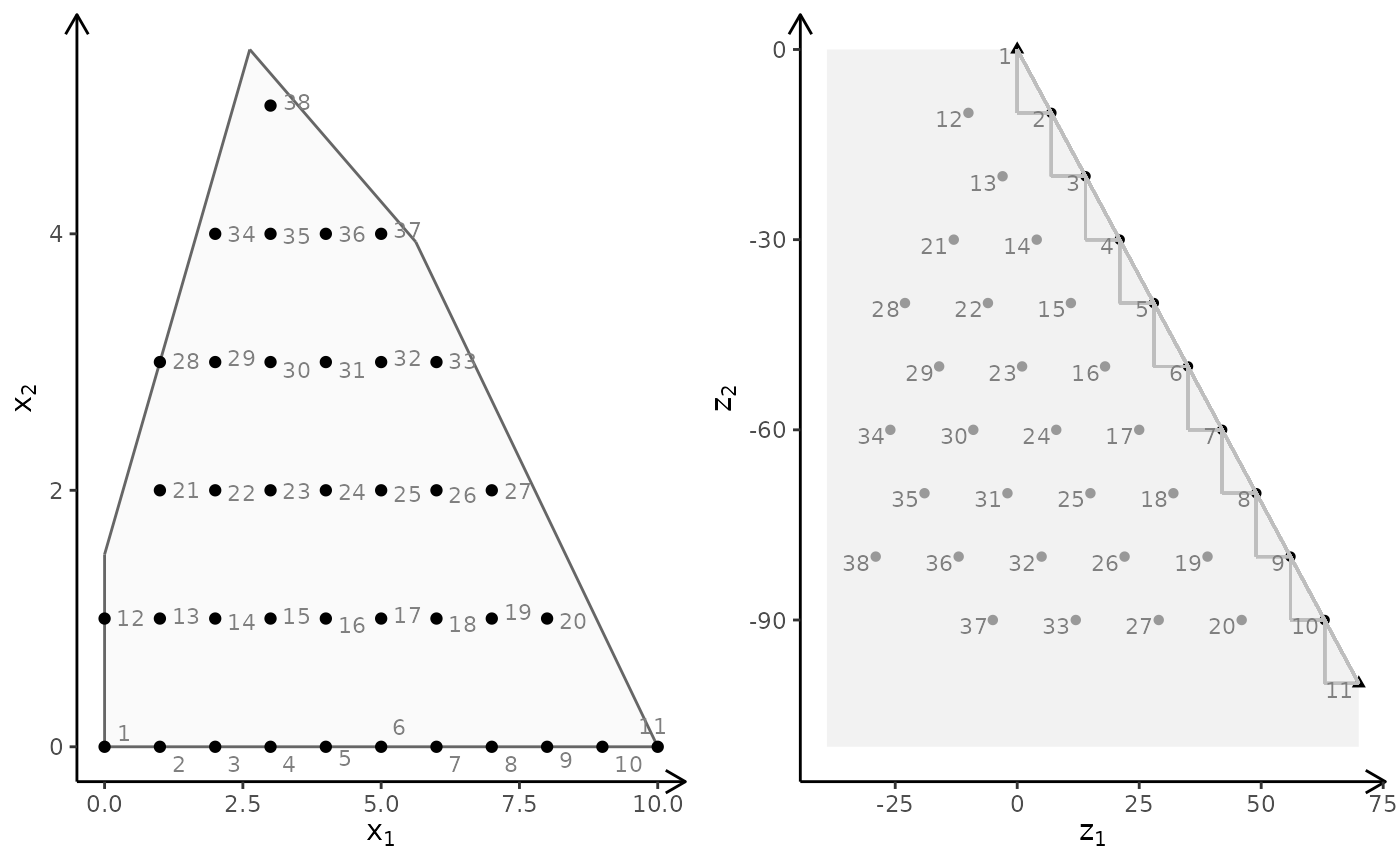
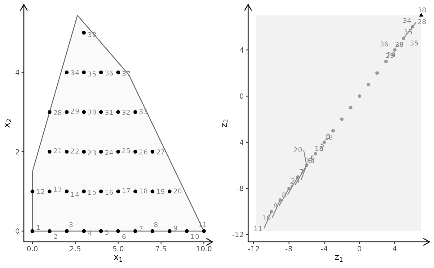
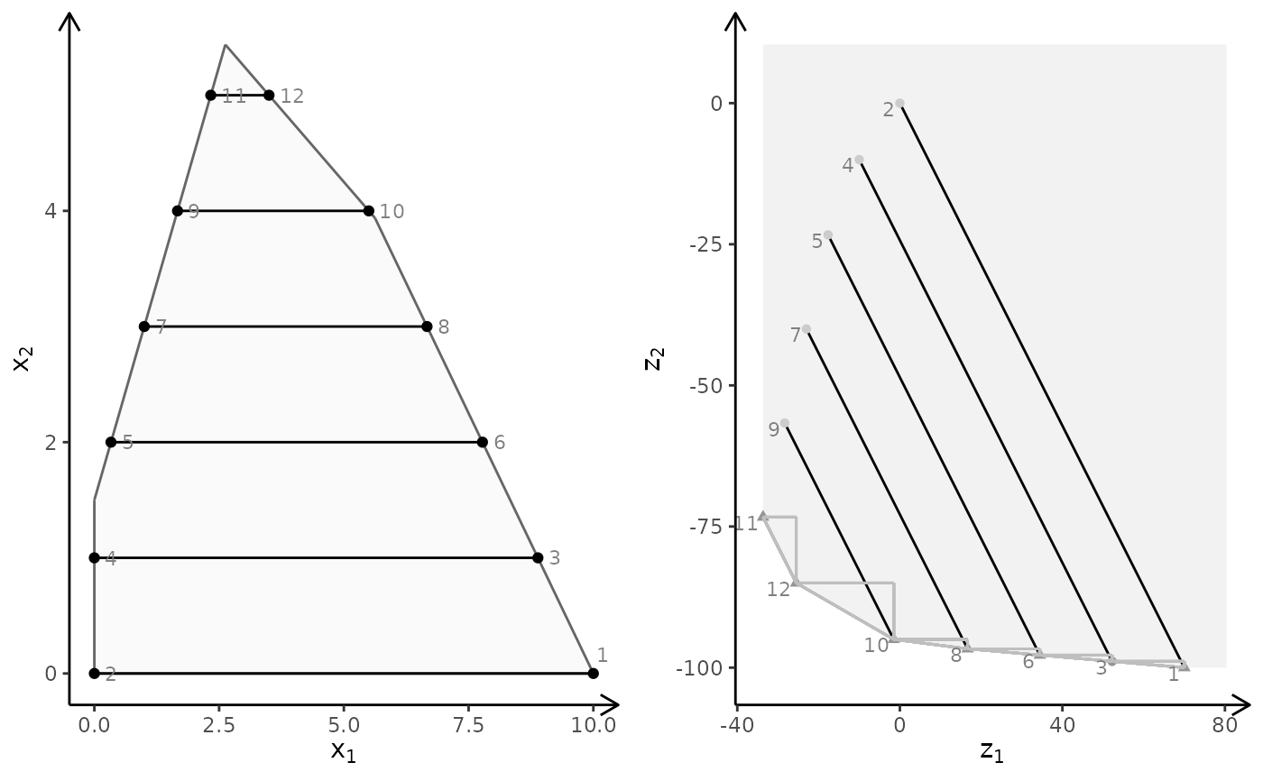
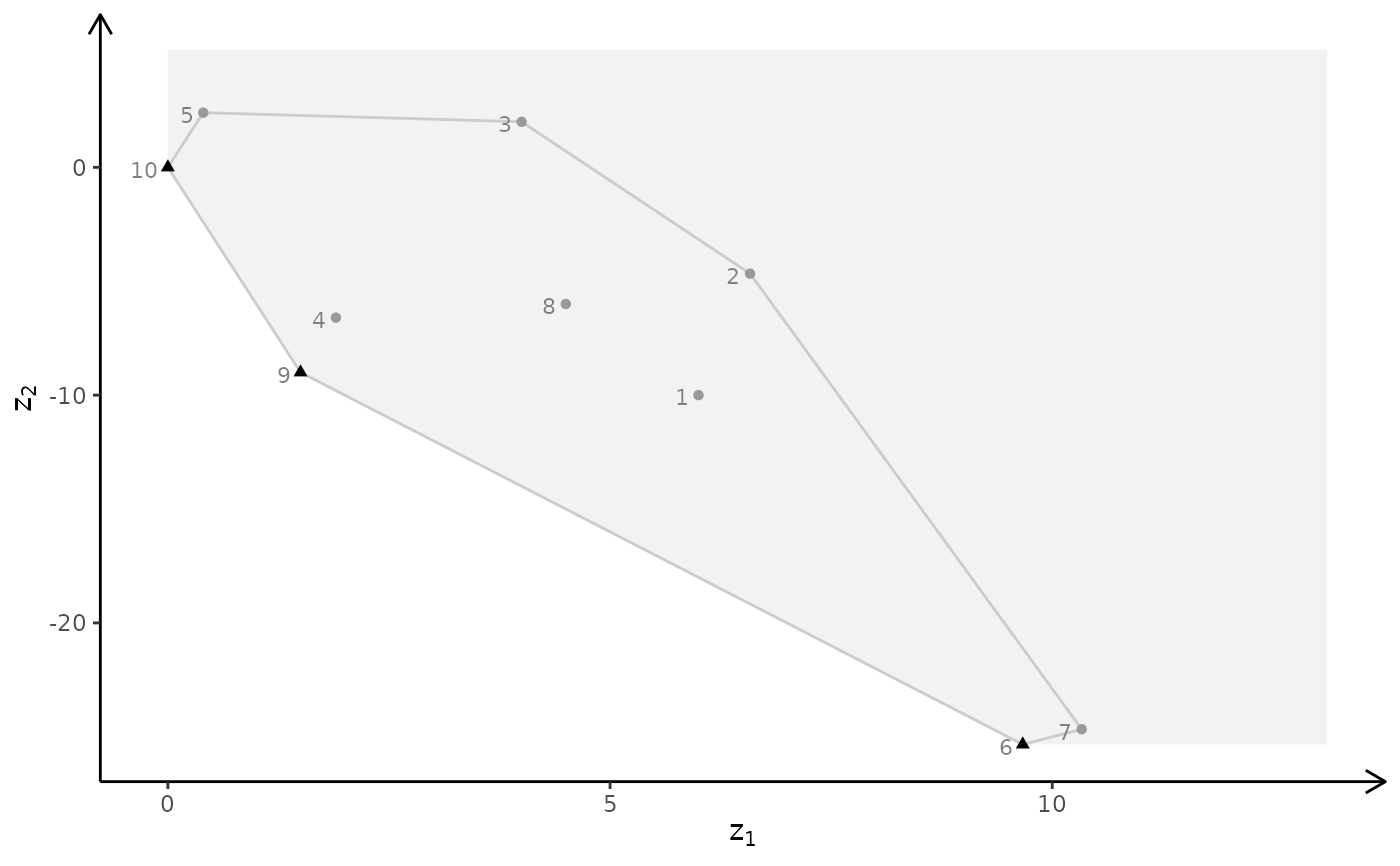
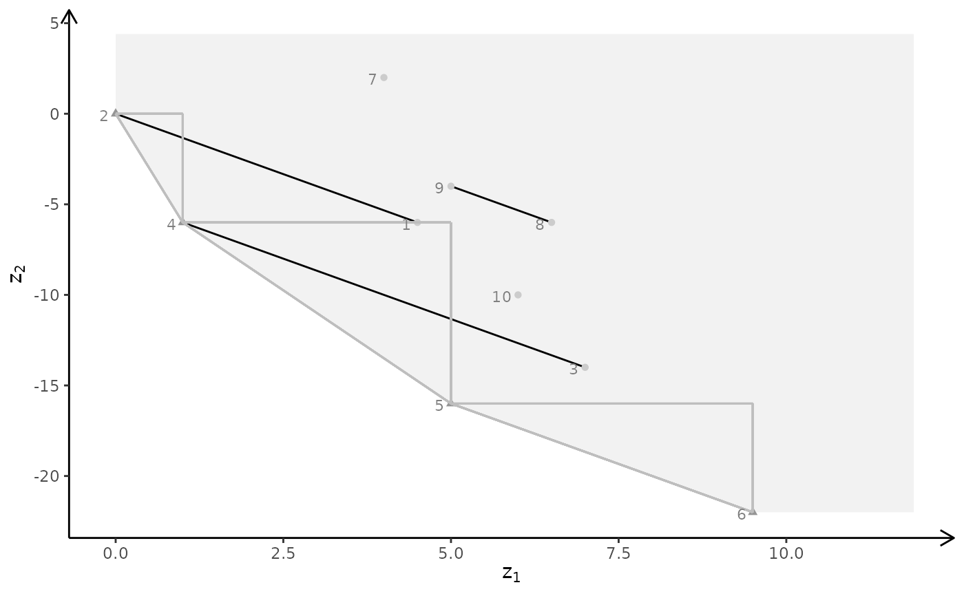
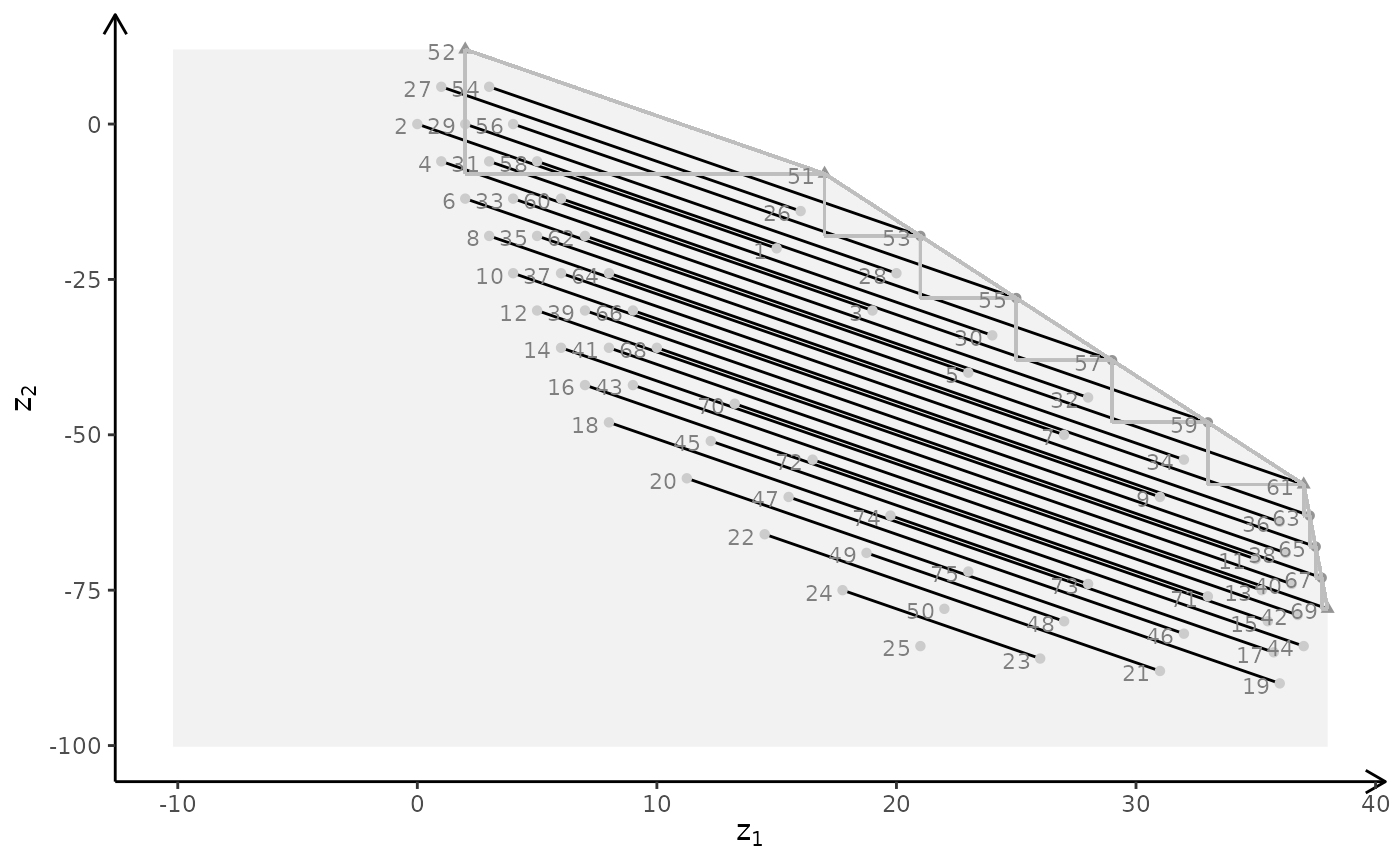
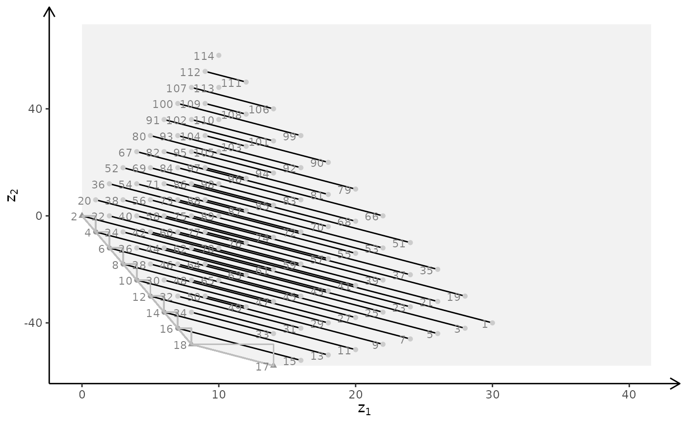
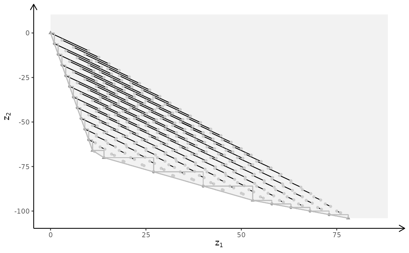
## ILP models with different criteria (maximize)
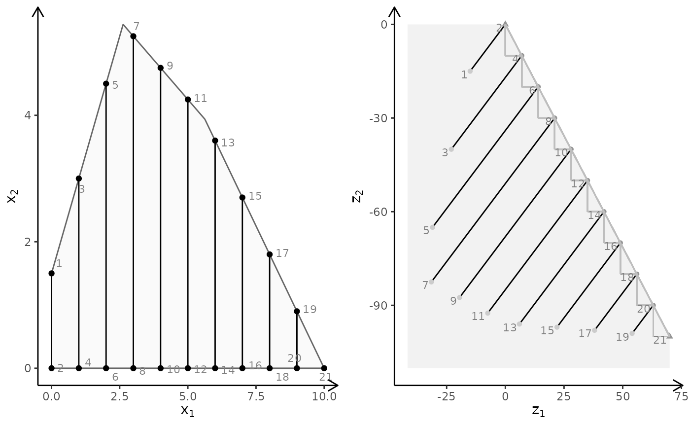
obj <- matrix(c(7, -10, -10, -10), nrow = 2)
plotBiObj2D(A, b, obj, type = rep("i", ncol(A)))
# \donttest{
## ILP models with different criteria (maximize)
obj <- matrix(c(7, -10, -10, -10), nrow = 2)
plotBiObj2D(A, b, obj, type = rep("i", ncol(A)))
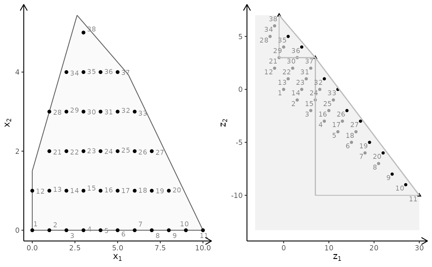
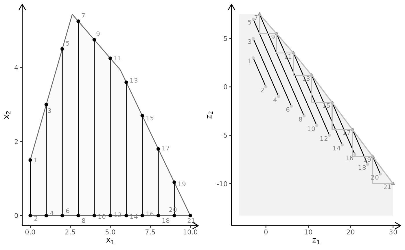
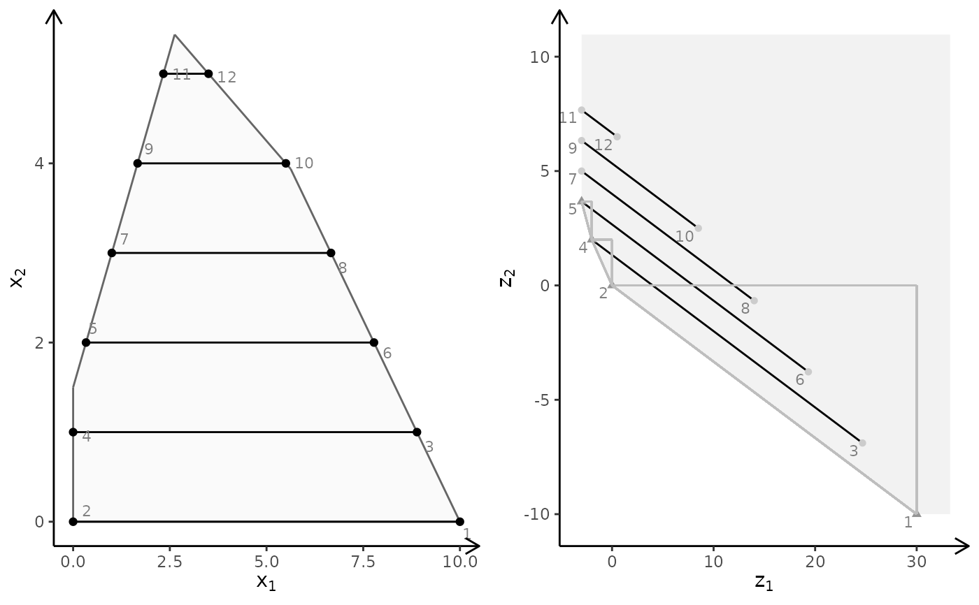
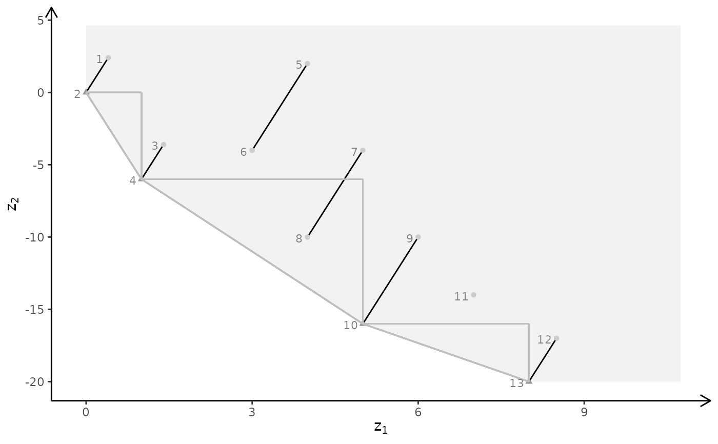
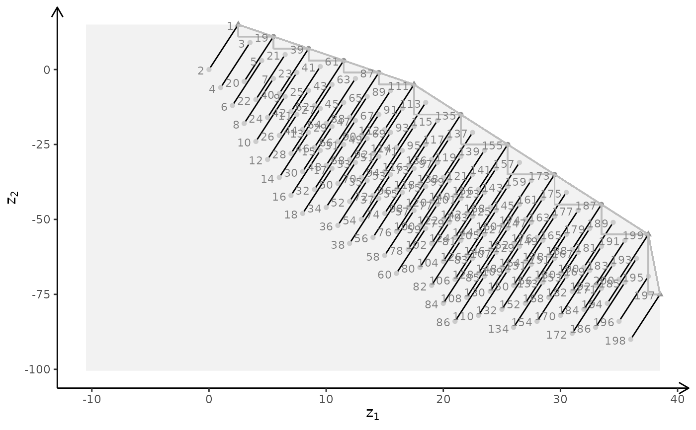
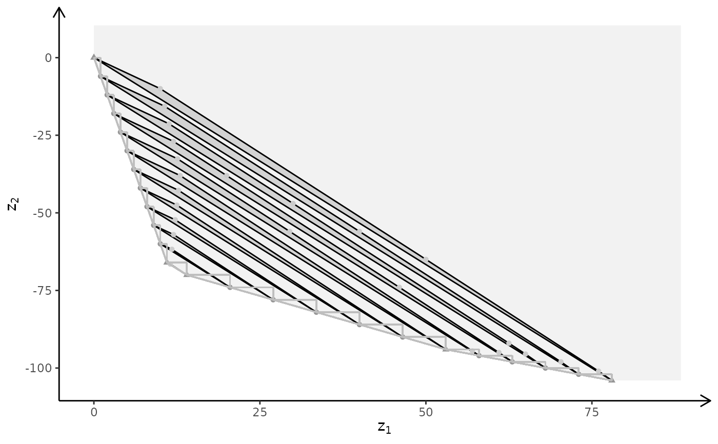
 obj <- matrix(c(3, -1, -2, 2), nrow = 2)
plotBiObj2D(A, b, obj, type = rep("i", ncol(A)))
obj <- matrix(c(3, -1, -2, 2), nrow = 2)
plotBiObj2D(A, b, obj, type = rep("i", ncol(A)))
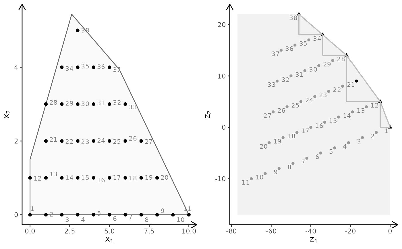
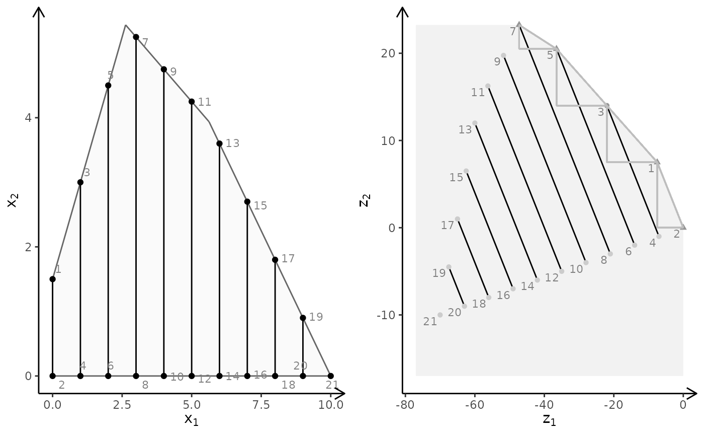
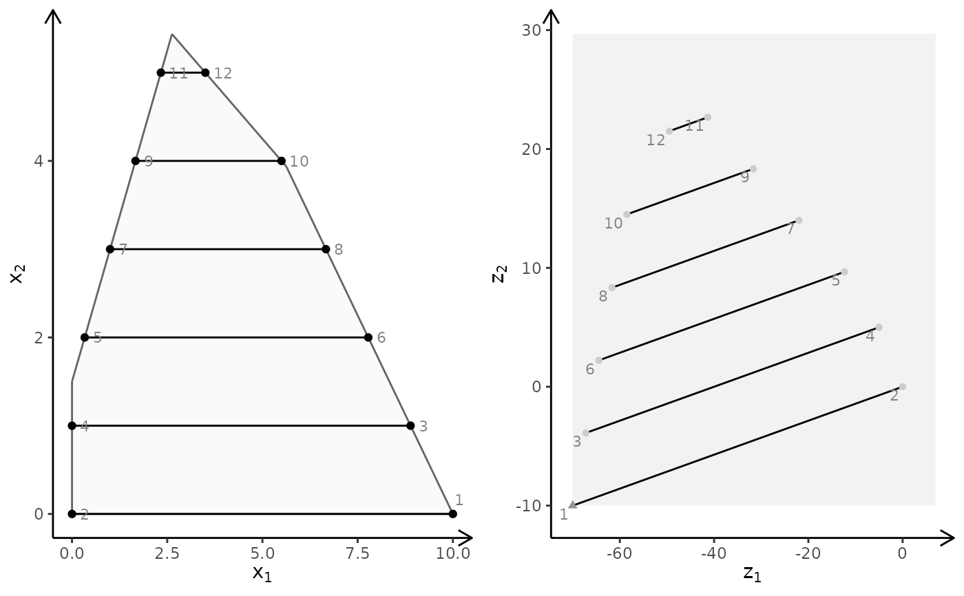
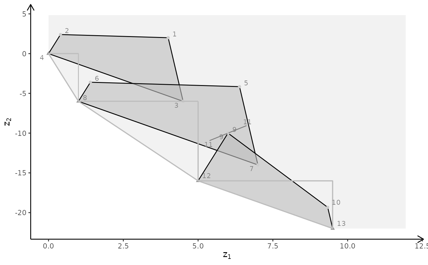
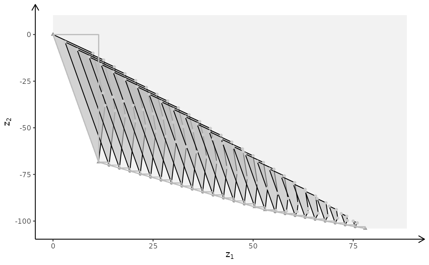
 obj <- matrix(c(-7, -1, -5, 5), nrow = 2)
plotBiObj2D(A, b, obj, type = rep("i", ncol(A)))
obj <- matrix(c(-7, -1, -5, 5), nrow = 2)
plotBiObj2D(A, b, obj, type = rep("i", ncol(A)))
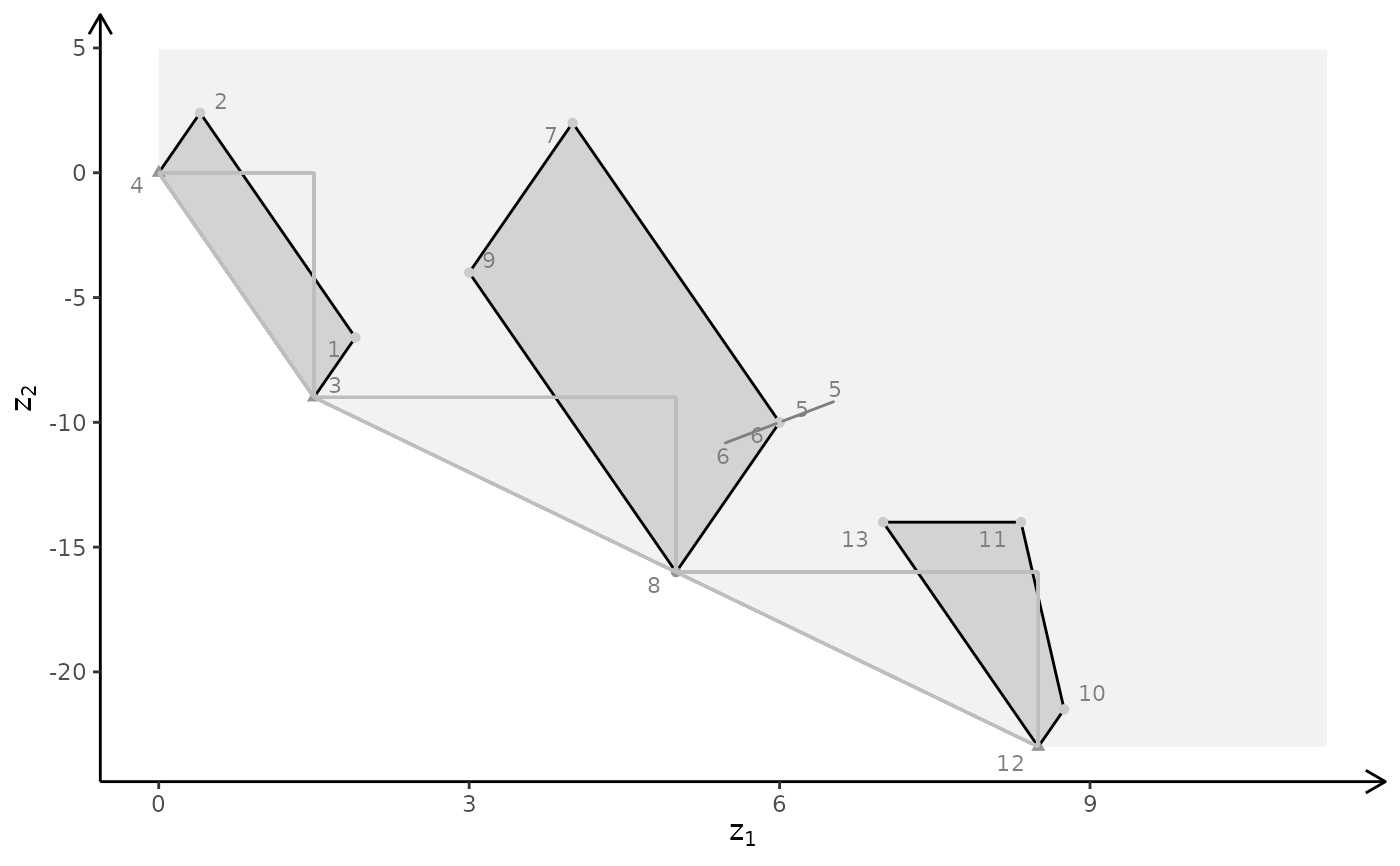
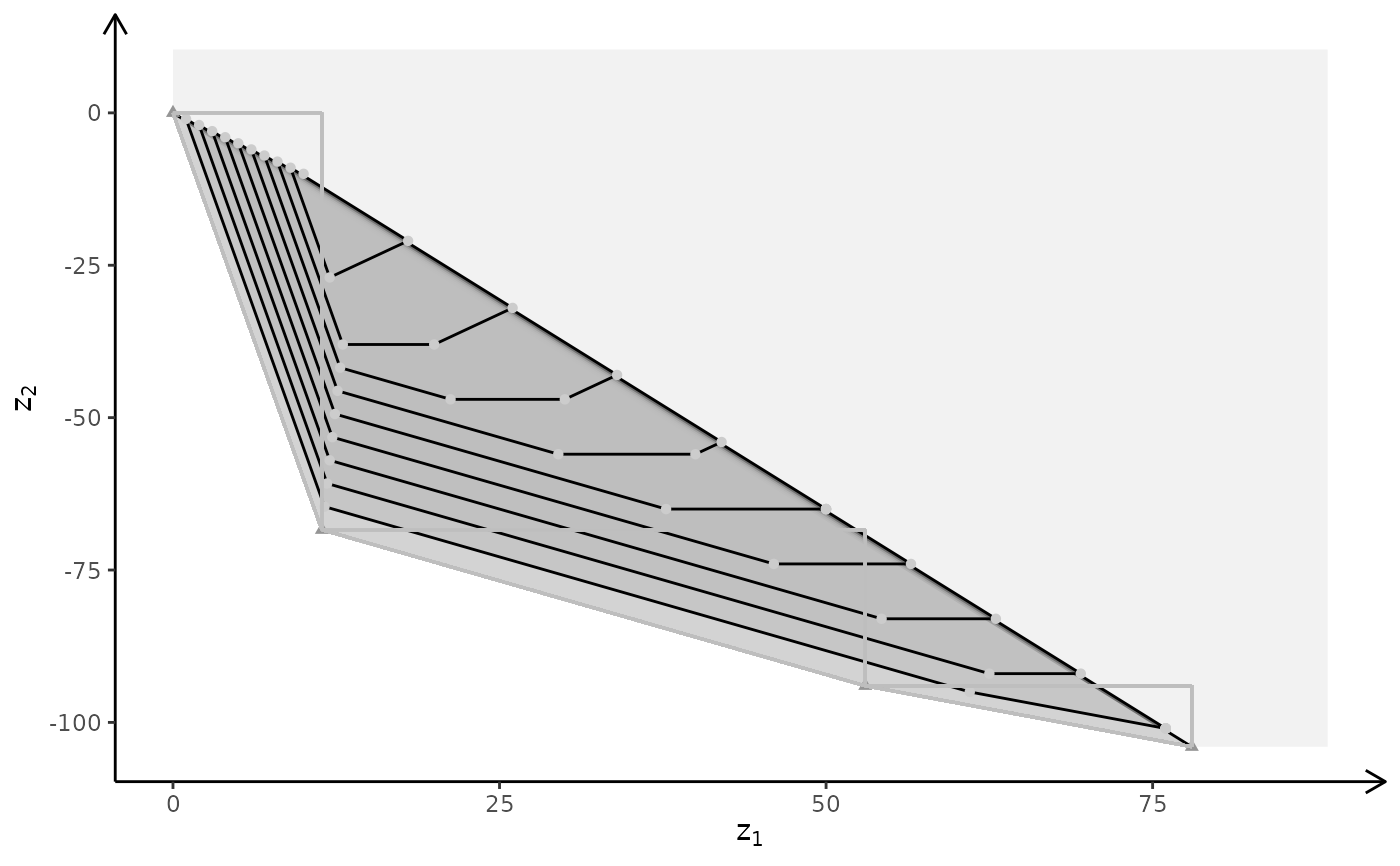
 obj <- matrix(c(-1, -1, 2, 2), nrow = 2)
plotBiObj2D(A, b, obj, type = rep("i", ncol(A)))
obj <- matrix(c(-1, -1, 2, 2), nrow = 2)
plotBiObj2D(A, b, obj, type = rep("i", ncol(A)))
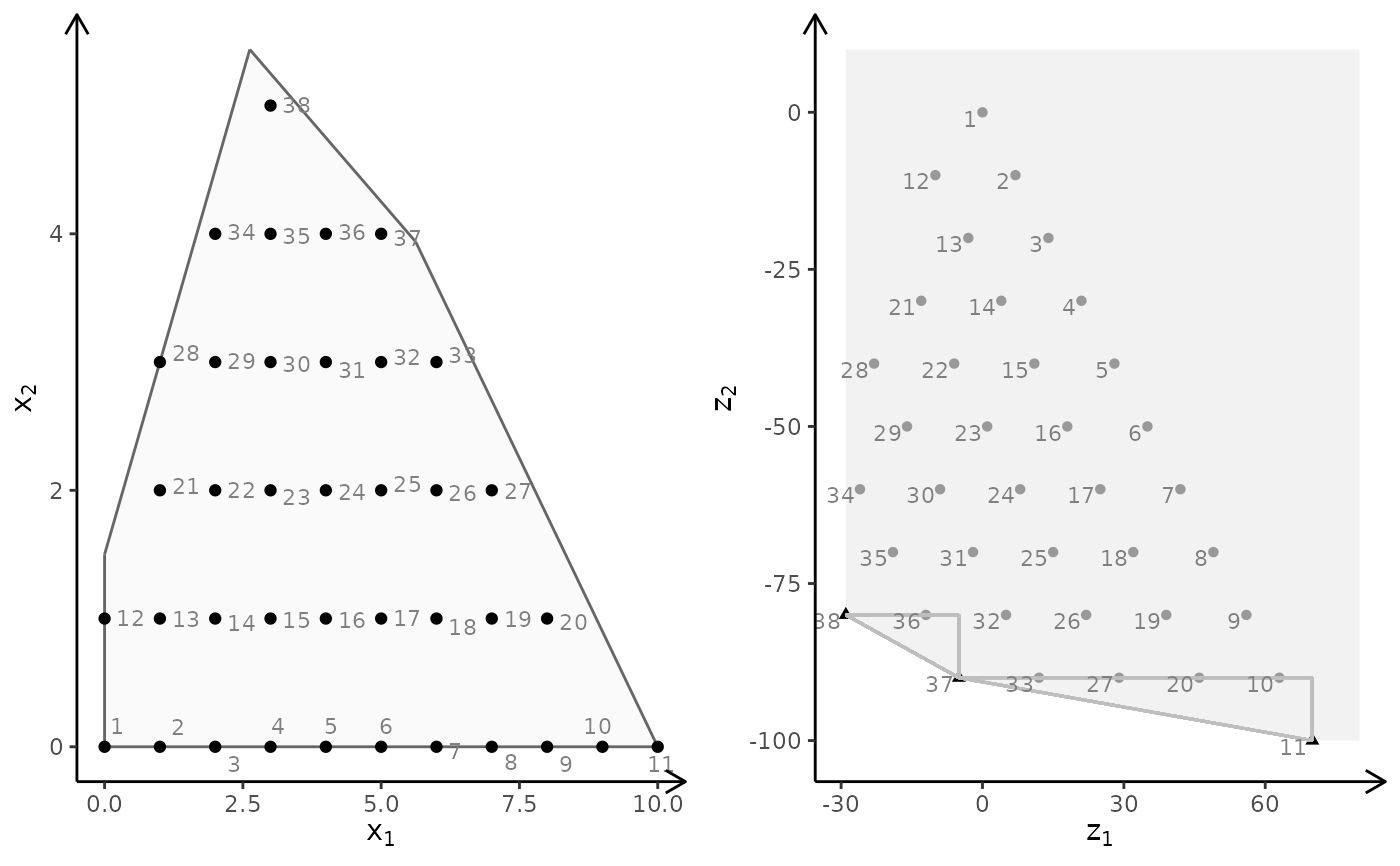
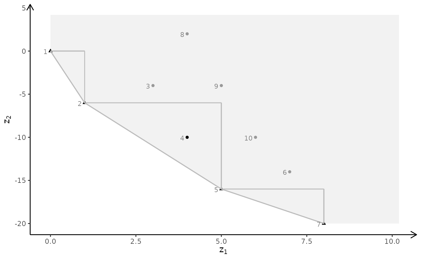
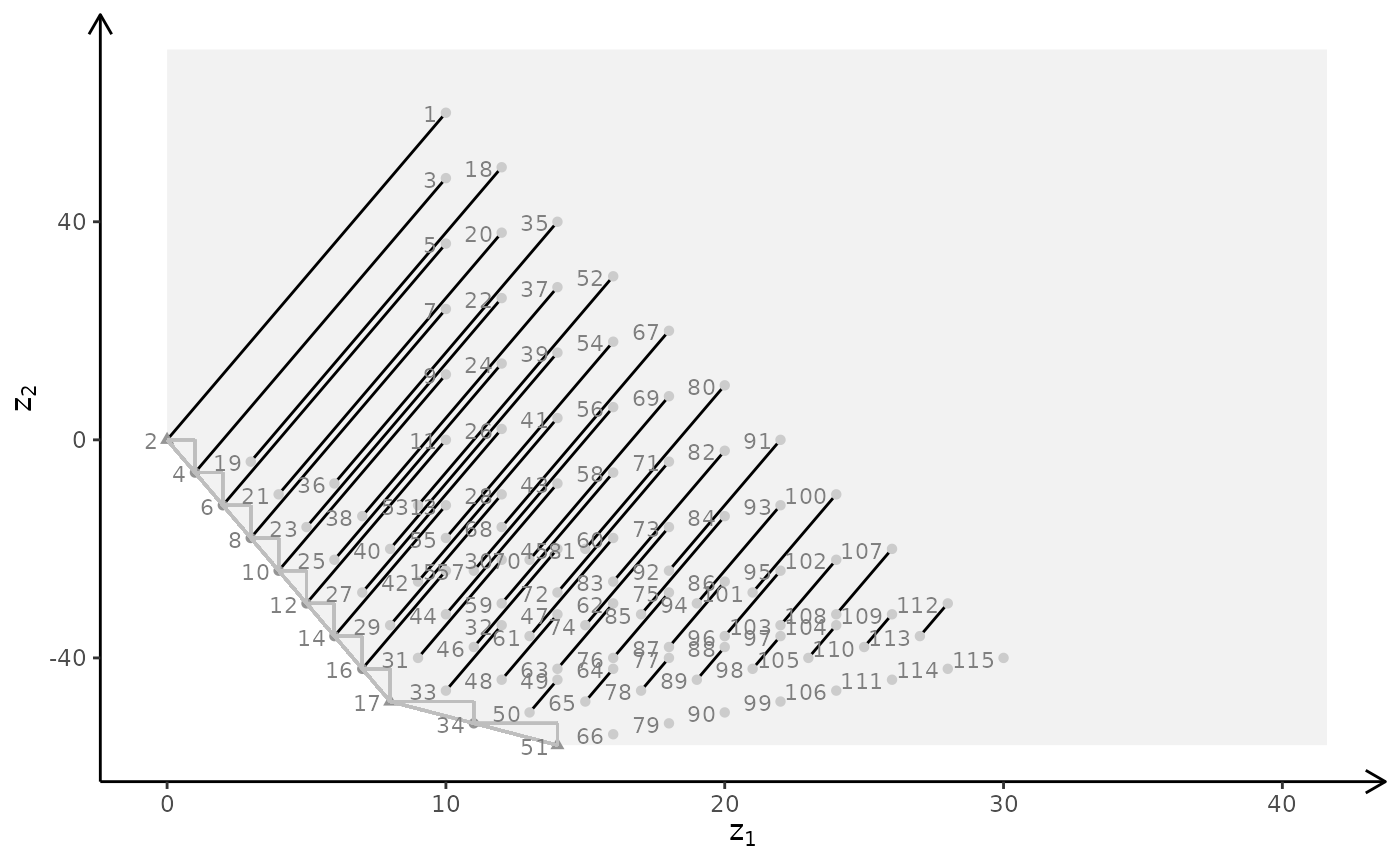
 ## ILP models with different criteria (minimize)
obj <- matrix(c(7, -10, -10, -10), nrow = 2)
plotBiObj2D(A, b, obj, type = rep("i", ncol(A)), crit = "min")
## ILP models with different criteria (minimize)
obj <- matrix(c(7, -10, -10, -10), nrow = 2)
plotBiObj2D(A, b, obj, type = rep("i", ncol(A)), crit = "min")
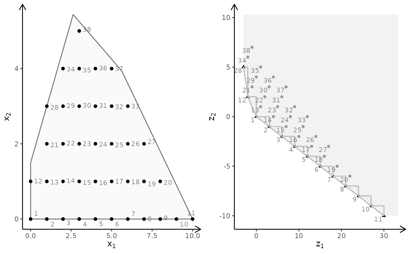
 obj <- matrix(c(3, -1, -2, 2), nrow = 2)
plotBiObj2D(A, b, obj, type = rep("i", ncol(A)), crit = "min")
obj <- matrix(c(3, -1, -2, 2), nrow = 2)
plotBiObj2D(A, b, obj, type = rep("i", ncol(A)), crit = "min")
 obj <- matrix(c(-7, -1, -5, 5), nrow = 2)
plotBiObj2D(A, b, obj, type = rep("i", ncol(A)), crit = "min")
obj <- matrix(c(-7, -1, -5, 5), nrow = 2)
plotBiObj2D(A, b, obj, type = rep("i", ncol(A)), crit = "min")
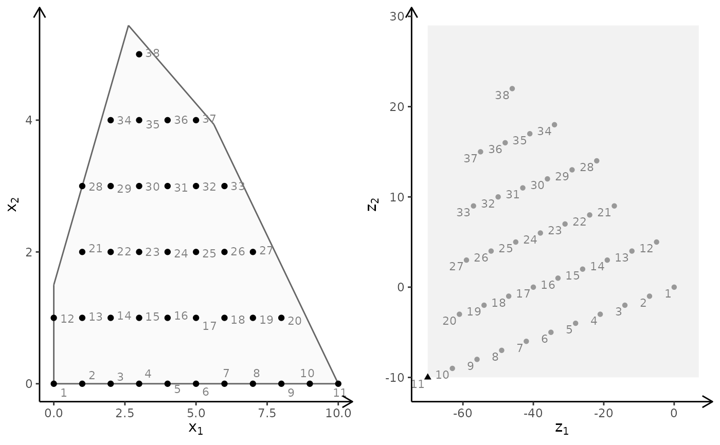 obj <- matrix(c(-1, -1, 2, 2), nrow = 2)
plotBiObj2D(A, b, obj, type = rep("i", ncol(A)), crit = "min")
obj <- matrix(c(-1, -1, 2, 2), nrow = 2)
plotBiObj2D(A, b, obj, type = rep("i", ncol(A)), crit = "min")
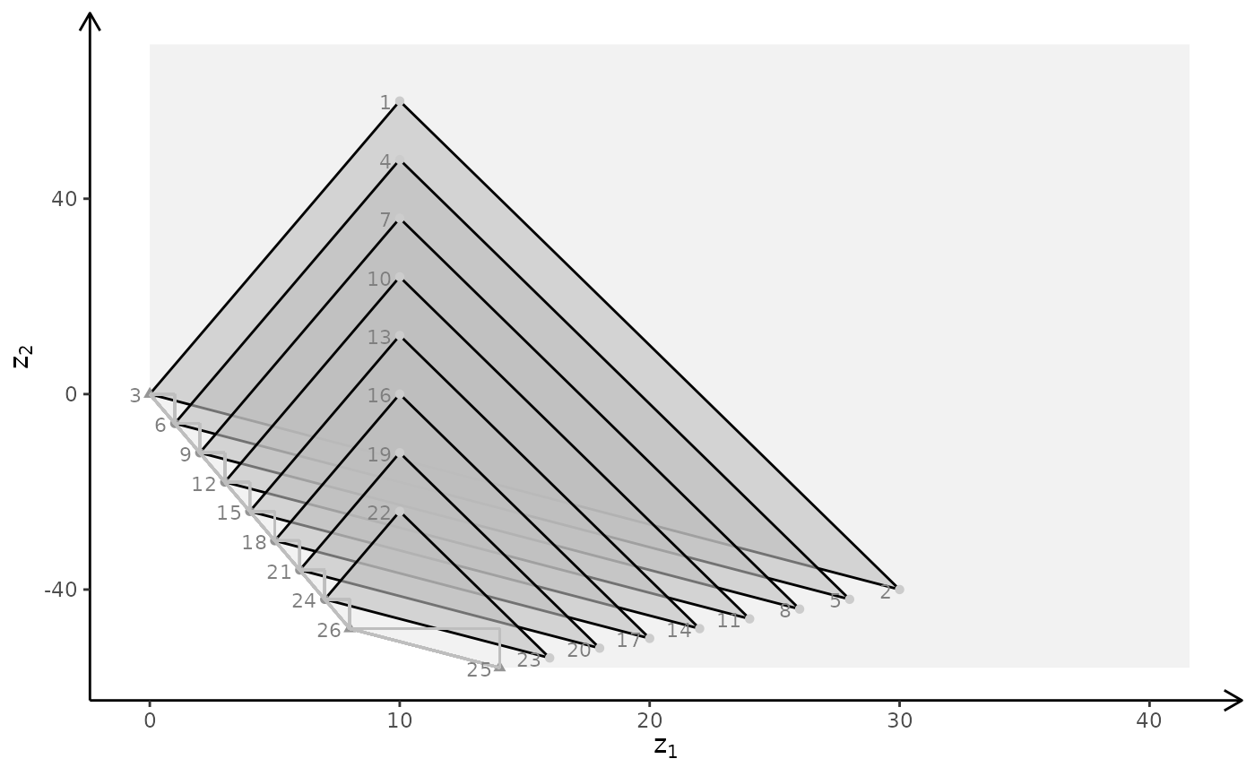
 # More examples
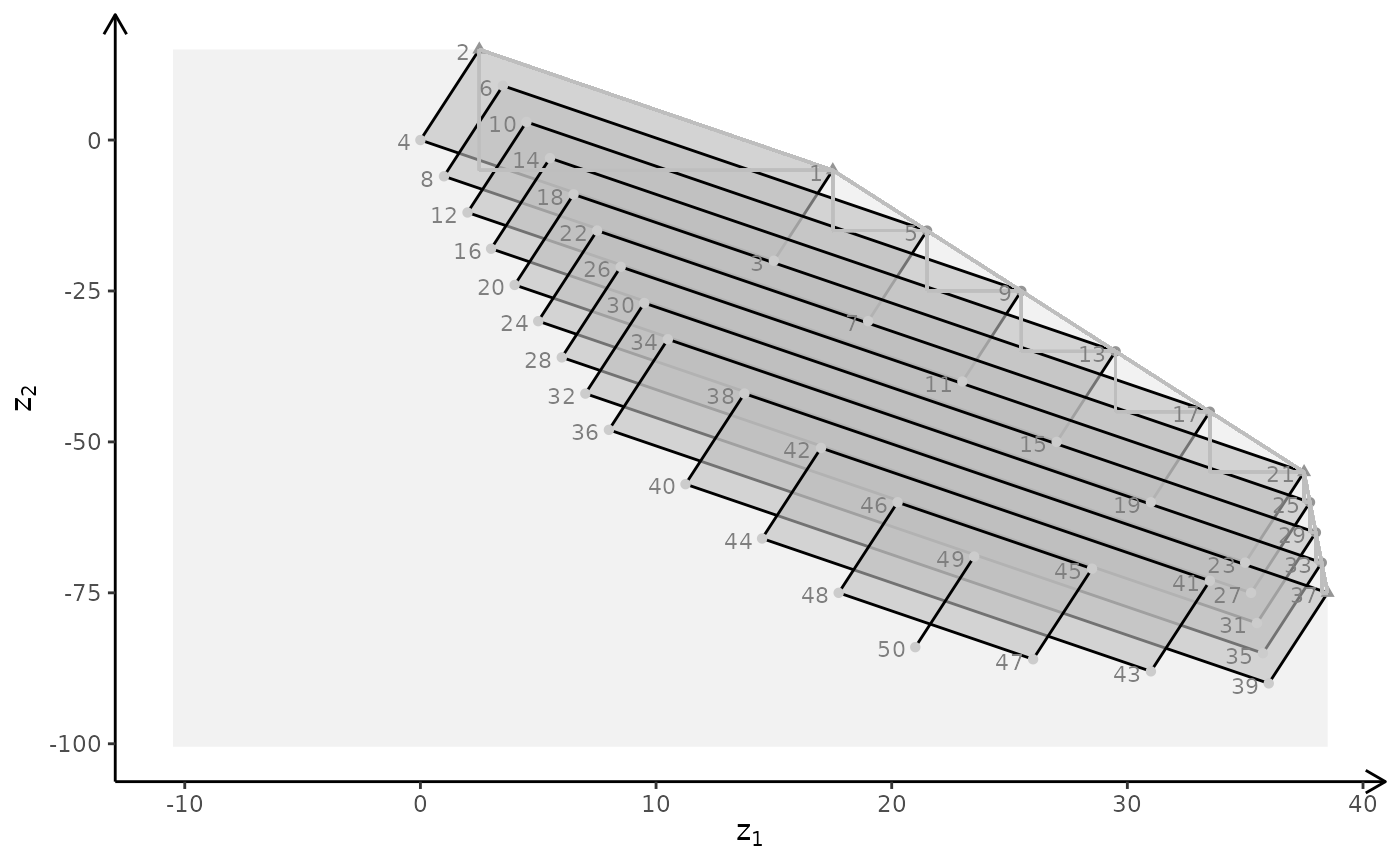
## MILP model (x1 integer) with different criteria (maximize)
obj <- matrix(c(7, -10, -10, -10), nrow = 2)
plotBiObj2D(A, b, obj, type = c("i", "c"))
# More examples
## MILP model (x1 integer) with different criteria (maximize)
obj <- matrix(c(7, -10, -10, -10), nrow = 2)
plotBiObj2D(A, b, obj, type = c("i", "c"))
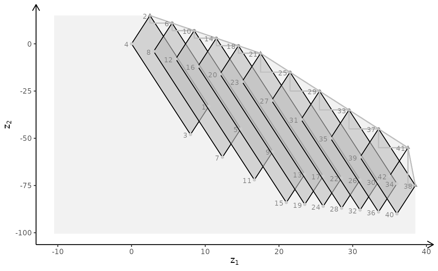
 obj <- matrix(c(3, -1, -2, 2), nrow = 2)
plotBiObj2D(A, b, obj, type = c("i", "c"))
obj <- matrix(c(3, -1, -2, 2), nrow = 2)
plotBiObj2D(A, b, obj, type = c("i", "c"))
 obj <- matrix(c(-7, -1, -5, 5), nrow = 2)
plotBiObj2D(A, b, obj, type = c("i", "c"))
obj <- matrix(c(-7, -1, -5, 5), nrow = 2)
plotBiObj2D(A, b, obj, type = c("i", "c"))
 obj <- matrix(c(-1, -1, 2, 2), nrow = 2)
plotBiObj2D(A, b, obj, type = c("i", "c"))
obj <- matrix(c(-1, -1, 2, 2), nrow = 2)
plotBiObj2D(A, b, obj, type = c("i", "c"))
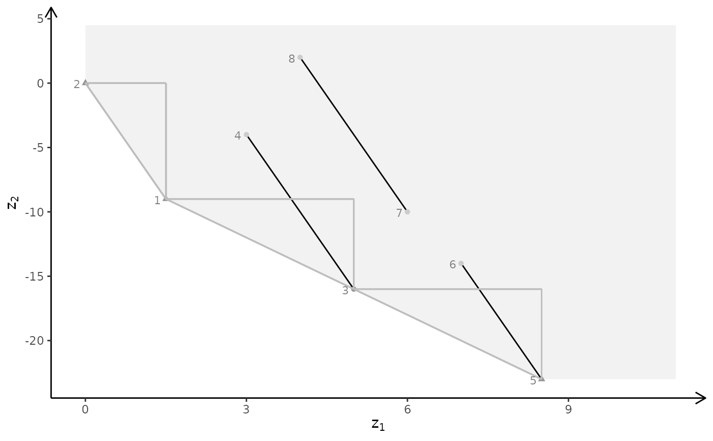
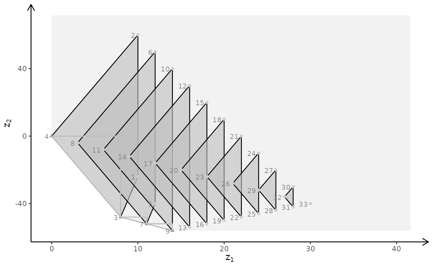
 ## MILP model (x2 integer) with different criteria (minimize)
obj <- matrix(c(7, -10, -10, -10), nrow = 2)
plotBiObj2D(A, b, obj, type = c("c", "i"), crit = "min")
## MILP model (x2 integer) with different criteria (minimize)
obj <- matrix(c(7, -10, -10, -10), nrow = 2)
plotBiObj2D(A, b, obj, type = c("c", "i"), crit = "min")
 obj <- matrix(c(3, -1, -2, 2), nrow = 2)
plotBiObj2D(A, b, obj, type = c("c", "i"), crit = "min")
obj <- matrix(c(3, -1, -2, 2), nrow = 2)
plotBiObj2D(A, b, obj, type = c("c", "i"), crit = "min")
 obj <- matrix(c(-7, -1, -5, 5), nrow = 2)
plotBiObj2D(A, b, obj, type = c("c", "i"), crit = "min")
obj <- matrix(c(-7, -1, -5, 5), nrow = 2)
plotBiObj2D(A, b, obj, type = c("c", "i"), crit = "min")
 obj <- matrix(c(-1, -1, 2, 2), nrow = 2)
plotBiObj2D(A, b, obj, type = c("c", "i"), crit = "min")
obj <- matrix(c(-1, -1, 2, 2), nrow = 2)
plotBiObj2D(A, b, obj, type = c("c", "i"), crit = "min")
 # }
### Set up 3D plot
# \donttest{
# Function for plotting the solution and criterion space in one plot (three variables)
plotBiObj3D <- function(A, b, obj,
type = rep("c", ncol(A)),
crit = "max",
faces = rep("c", ncol(A)),
plotFaces = TRUE,
plotFeasible = TRUE,
plotOptimum = FALSE,
labels = "numb",
addTriangles = TRUE,
addHull = TRUE)
{
plotPolytope(A, b, type = type, crit = crit, faces = faces, plotFaces = plotFaces,
plotFeasible = plotFeasible, plotOptimum = plotOptimum, labels = labels)
plotCriterion2D(A, b, obj, type = type, crit = crit, addTriangles = addTriangles,
addHull = addHull, plotFeasible = plotFeasible, labels = labels)
}
### Bi-objective problem with three variables
loadView <- function(fname = "view.RData", v = NULL) {
if (!is.null(v)) {
rgl::view3d(userMatrix = v)
} else {
if (file.exists(fname)) {
load(fname)
rgl::view3d(userMatrix = view)
} else {
warning(paste0("Can'TRUE load view in file ", fname, "!"))
}
}
}
## Ex
view <- matrix( c(-0.452365815639496, -0.446501553058624, 0.77201122045517, 0, 0.886364221572876,
-0.320795893669128, 0.333835482597351, 0, 0.0986008867621422, 0.835299551486969,
0.540881276130676, 0, 0, 0, 0, 1), nc = 4)
loadView(v = view)
# }
### Set up 3D plot
# \donttest{
# Function for plotting the solution and criterion space in one plot (three variables)
plotBiObj3D <- function(A, b, obj,
type = rep("c", ncol(A)),
crit = "max",
faces = rep("c", ncol(A)),
plotFaces = TRUE,
plotFeasible = TRUE,
plotOptimum = FALSE,
labels = "numb",
addTriangles = TRUE,
addHull = TRUE)
{
plotPolytope(A, b, type = type, crit = crit, faces = faces, plotFaces = plotFaces,
plotFeasible = plotFeasible, plotOptimum = plotOptimum, labels = labels)
plotCriterion2D(A, b, obj, type = type, crit = crit, addTriangles = addTriangles,
addHull = addHull, plotFeasible = plotFeasible, labels = labels)
}
### Bi-objective problem with three variables
loadView <- function(fname = "view.RData", v = NULL) {
if (!is.null(v)) {
rgl::view3d(userMatrix = v)
} else {
if (file.exists(fname)) {
load(fname)
rgl::view3d(userMatrix = view)
} else {
warning(paste0("Can'TRUE load view in file ", fname, "!"))
}
}
}
## Ex
view <- matrix( c(-0.452365815639496, -0.446501553058624, 0.77201122045517, 0, 0.886364221572876,
-0.320795893669128, 0.333835482597351, 0, 0.0986008867621422, 0.835299551486969,
0.540881276130676, 0, 0, 0, 0, 1), nc = 4)
loadView(v = view)
3D plot
Ab <- matrix( c(
1, 1, 2, 5,
2, -1, 0, 3,
-1, 2, 1, 3,
0, -3, 5, 2
), nc = 4, byrow = TRUE)
A <- Ab[,1:3]
b <- Ab[,4]
obj <- matrix(c(1, -6, 3, -4, 1, 6), nrow = 2)
# LP model
plotBiObj3D(A, b, obj, crit = "min", addTriangles = FALSE)
 # ILP model
plotBiObj3D(A, b, obj, type = c("i","i","i"), crit = "min")
# ILP model
plotBiObj3D(A, b, obj, type = c("i","i","i"), crit = "min")
 # MILP model
plotBiObj3D(A, b, obj, type = c("c","i","i"), crit = "min")
# MILP model
plotBiObj3D(A, b, obj, type = c("c","i","i"), crit = "min")
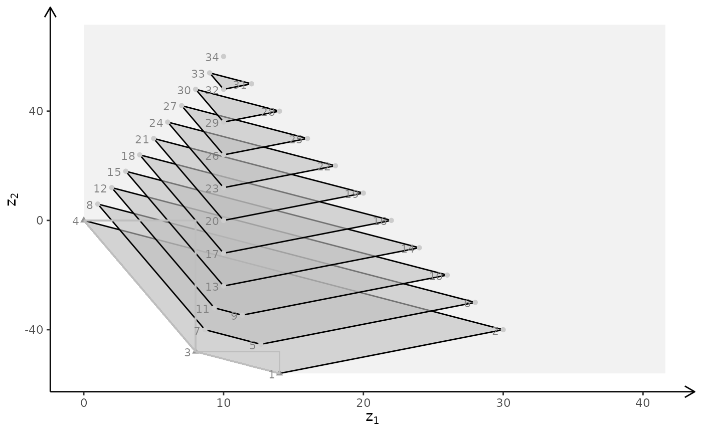
 plotBiObj3D(A, b, obj, type = c("i","c","i"), crit = "min")
 plotBiObj3D(A, b, obj, type = c("i","i","c"), crit = "min")
 plotBiObj3D(A, b, obj, type = c("i","c","c"), crit = "min")
 plotBiObj3D(A, b, obj, type = c("c","i","c"), crit = "min")
 plotBiObj3D(A, b, obj, type = c("c","c","i"), crit = "min")
 ## Ex
view <- matrix( c(0.976349174976349, -0.202332556247711, 0.0761845782399178, 0, 0.0903248339891434,
0.701892614364624, 0.706531345844269, 0, -0.196427255868912, -0.682940244674683,
0.703568696975708, 0, 0, 0, 0, 1), nc = 4)
loadView(v = view)
## Ex
view <- matrix( c(0.976349174976349, -0.202332556247711, 0.0761845782399178, 0, 0.0903248339891434,
0.701892614364624, 0.706531345844269, 0, -0.196427255868912, -0.682940244674683,
0.703568696975708, 0, 0, 0, 0, 1), nc = 4)
loadView(v = view)
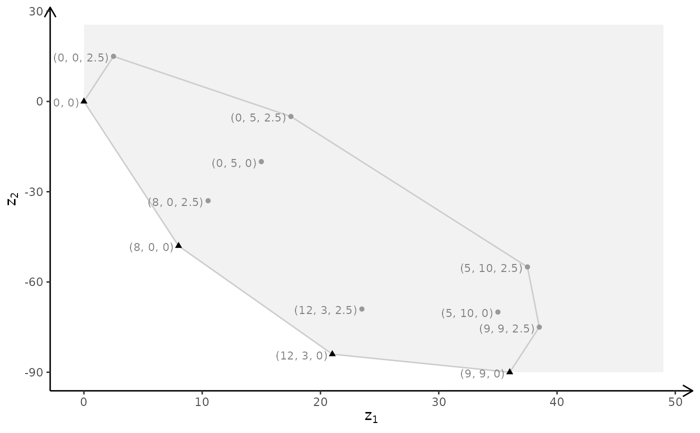
3D plot
A <- matrix( c(
-1, 1, 0,
1, 4, 0,
2, 1, 0,
3, -4, 0,
0, 0, 4
), nc = 3, byrow = TRUE)
b <- c(5, 45, 27, 24, 10)
obj <- matrix(c(1, -6, 3, -4, 1, 6), nrow = 2)
# LP model
plotBiObj3D(A, b, obj, crit = "min", addTriangles = FALSE, labels = "coord")
 # ILP model
plotBiObj3D(A, b, obj, type = c("i","i","i"))
# ILP model
plotBiObj3D(A, b, obj, type = c("i","i","i"))
 # MILP model
plotBiObj3D(A, b, obj, type = c("c","i","i"))
# MILP model
plotBiObj3D(A, b, obj, type = c("c","i","i"))
 plotBiObj3D(A, b, obj, type = c("i","c","i"), plotFaces = FALSE)
 plotBiObj3D(A, b, obj, type = c("i","i","c"))
 plotBiObj3D(A, b, obj, type = c("i","c","c"), plotFaces = FALSE)
 plotBiObj3D(A, b, obj, type = c("c","i","c"), plotFaces = FALSE)
 plotBiObj3D(A, b, obj, type = c("c","c","i"))
 ## Ex
view <- matrix( c(-0.812462985515594, -0.029454167932272, 0.582268416881561, 0, 0.579295456409454,
-0.153386667370796, 0.800555109977722, 0, 0.0657325685024261, 0.987727105617523,
0.14168381690979, 0, 0, 0, 0, 1), nc = 4)
loadView(v = view)
## Ex
view <- matrix( c(-0.812462985515594, -0.029454167932272, 0.582268416881561, 0, 0.579295456409454,
-0.153386667370796, 0.800555109977722, 0, 0.0657325685024261, 0.987727105617523,
0.14168381690979, 0, 0, 0, 0, 1), nc = 4)
loadView(v = view)
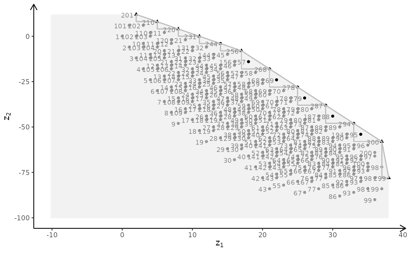
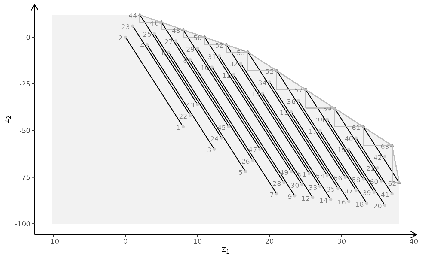
3D plot
A <- matrix( c(
1, 1, 1,
3, 0, 1
), nc = 3, byrow = TRUE)
b <- c(10, 24)
obj <- matrix(c(1, -6, 3, -4, 1, 6), nrow = 2)
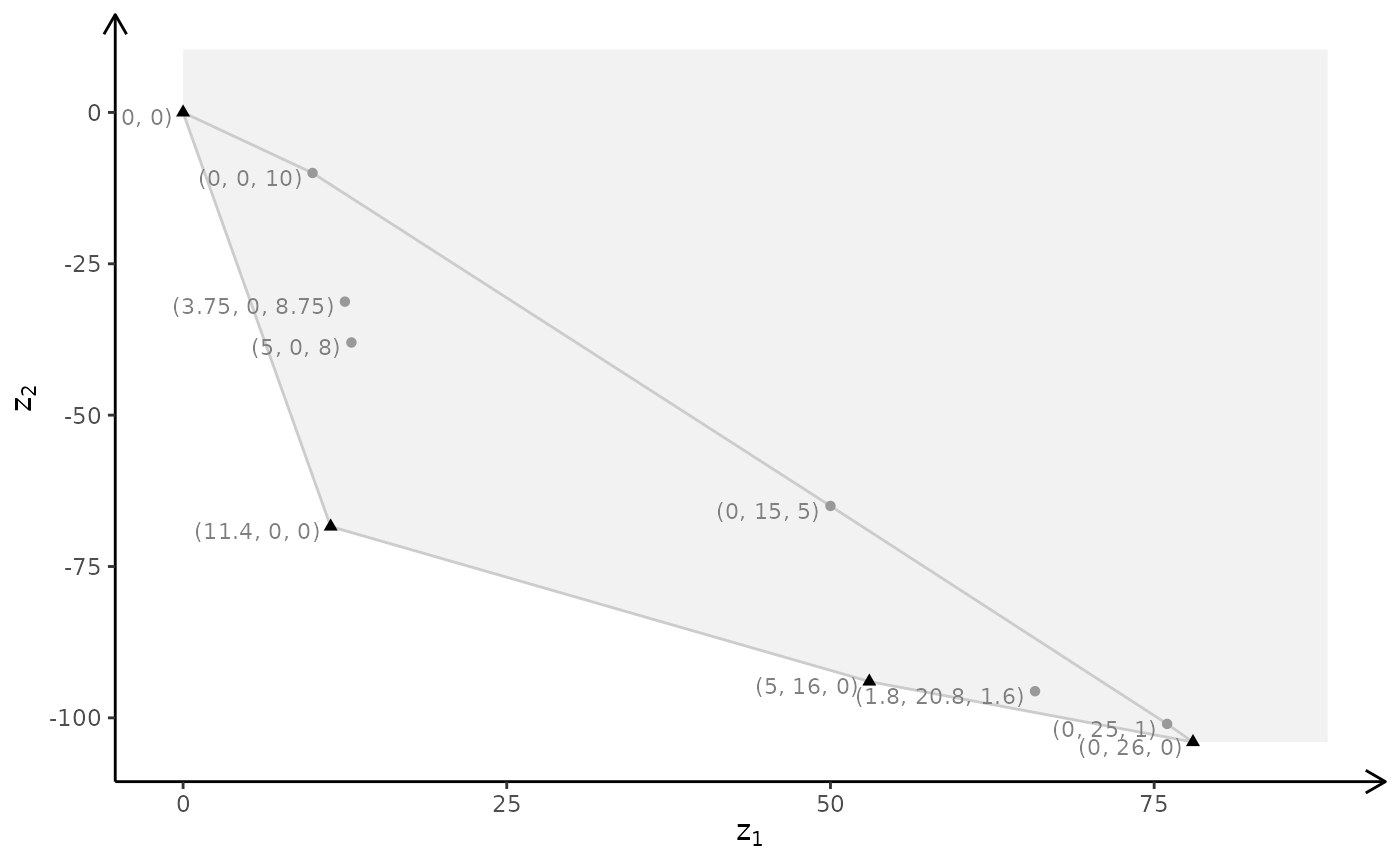
# LP model
plotBiObj3D(A, b, obj, crit = "min", addTriangles = FALSE, labels = "coord")
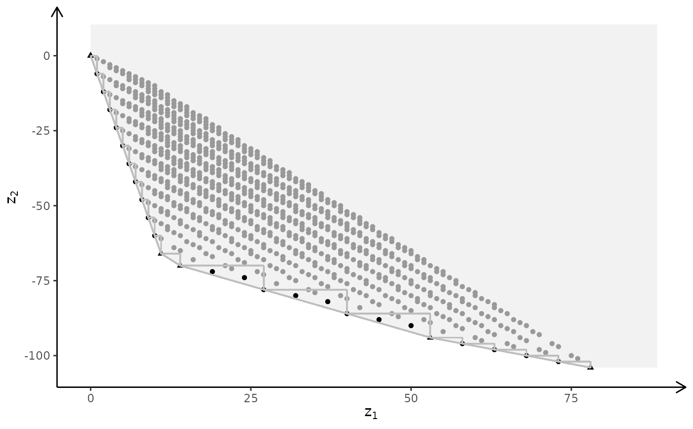
 # ILP model
plotBiObj3D(A, b, obj, type = c("i","i","i"), crit = "min", labels = "n")
# ILP model
plotBiObj3D(A, b, obj, type = c("i","i","i"), crit = "min", labels = "n")
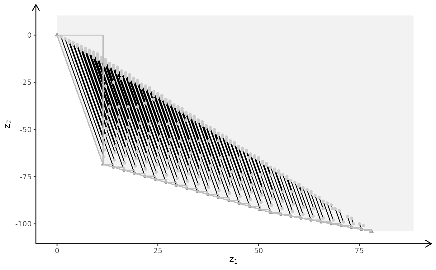
 # MILP model
plotBiObj3D(A, b, obj, type = c("c","i","i"), crit = "min")
# MILP model
plotBiObj3D(A, b, obj, type = c("c","i","i"), crit = "min")
 plotBiObj3D(A, b, obj, type = c("i","c","i"), crit = "min")
 plotBiObj3D(A, b, obj, type = c("i","i","c"), crit = "min")
 plotBiObj3D(A, b, obj, type = c("i","c","c"), crit = "min")
 plotBiObj3D(A, b, obj, type = c("c","i","c"), crit = "min", plotFaces = FALSE)
 plotBiObj3D(A, b, obj, type = c("c","c","i"), crit = "min", plotFaces = FALSE)
 ## Ex
view <- matrix( c(-0.412063330411911, -0.228006735444069, 0.882166087627411, 0, 0.910147845745087,
-0.0574885793030262, 0.410274744033813, 0, -0.042830865830183, 0.97196090221405,
0.231208890676498, 0, 0, 0, 0, 1), nc = 4)
loadView(v = view)
## Ex
view <- matrix( c(-0.412063330411911, -0.228006735444069, 0.882166087627411, 0, 0.910147845745087,
-0.0574885793030262, 0.410274744033813, 0, -0.042830865830183, 0.97196090221405,
0.231208890676498, 0, 0, 0, 0, 1), nc = 4)
loadView(v = view)
3D plot
A <- matrix( c(
3, 2, 5,
2, 1, 1,
1, 1, 3,
5, 2, 4
), nc = 3, byrow = TRUE)
b <- c(55, 26, 30, 57)
obj <- matrix(c(1, -6, 3, -4, 1, -1), nrow = 2)
# LP model
plotBiObj3D(A, b, obj, crit = "min", addTriangles = FALSE, labels = "coord")
#> Warning: edge not found:1 2
 # ILP model
plotBiObj3D(A, b, obj, type = c("i","i","i"), crit = "min", labels = "n")
#> Warning: edge not found:1 2
# ILP model
plotBiObj3D(A, b, obj, type = c("i","i","i"), crit = "min", labels = "n")
#> Warning: edge not found:1 2
 # MILP model
plotBiObj3D(A, b, obj, type = c("c","i","i"), crit = "min", labels = "n")
#> Warning: edge not found:1 2
# MILP model
plotBiObj3D(A, b, obj, type = c("c","i","i"), crit = "min", labels = "n")
#> Warning: edge not found:1 2
 plotBiObj3D(A, b, obj, type = c("i","c","i"), crit = "min", labels = "n", plotFaces = FALSE)
 plotBiObj3D(A, b, obj, type = c("i","i","c"), crit = "min", labels = "n")
#> Warning: edge not found:1 2
plotBiObj3D(A, b, obj, type = c("i","i","c"), crit = "min", labels = "n")
#> Warning: edge not found:1 2
 plotBiObj3D(A, b, obj, type = c("i","c","c"), crit = "min", labels = "n")
#> Warning: edge not found:1 2
plotBiObj3D(A, b, obj, type = c("i","c","c"), crit = "min", labels = "n")
#> Warning: edge not found:1 2
 plotBiObj3D(A, b, obj, type = c("c","i","c"), crit = "min", labels = "n", plotFaces = FALSE)
 plotBiObj3D(A, b, obj, type = c("c","c","i"), crit = "min", labels = "n")
#> Warning: edge not found:1 2
plotBiObj3D(A, b, obj, type = c("c","c","i"), crit = "min", labels = "n")
#> Warning: edge not found:1 2
 # }
# }