An infinite-horizon HMDP
Lars Relund lars@relund.dk
2026-06-22
Source:vignettes/infinite-hmdp.Rmd
infinite-hmdp.RmdThe MDP2 package in R is a package for solving Markov
decision processes (MDPs) with discrete time-steps, states and actions.
Both traditional MDPs (Puterman 1994),
semi-Markov decision processes (semi-MDPs) (Tijms
2003) and hierarchical-MDPs (HMDPs) (Kristensen and Jørgensen 2000) can be solved
under a finite and infinite time-horizon.
The package implement well-known algorithms such as policy iteration
and value iteration under different criteria e.g. average reward per
time unit and expected total discounted reward. The model is stored
using an underlying data structure based on the state-expanded
directed hypergraph of the MDP (Nielsen and
Kristensen (2006)) implemented in C++ for fast
running times.
Building and solving an MDP is done in two steps. First, the MDP is built and saved in a set of binary files. Next, you load the MDP into memory from the binary files and apply various algorithms to the model.
For building the MDP models see vignette("building"). In
this vignette we focus on the second step, i.e. finding the optimal
policy. Here we consider an infinite-horizon HMDP.
An infinite-horizon HMDP
A hierarchical MDP is an MDP with parameters defined in a special
way, but nevertheless in accordance with all usual rules and conditions
relating to such processes (Kristensen and
Jørgensen (2000)). The basic idea of the hierarchical structure
is that stages of the process can be expanded to a so-called child
process, which again may expand stages further to new child
processes leading to multiple levels. To illustrate consider the HMDP
shown in the figure below. The process has three levels. At
Level 2 we have a set of finite-horizon semi-MDPs (one for
each oval box) which all can be represented using a state-expanded
hypergraph (hyperarcs not shown, only hyperarcs connecting processes are
shown). A semi-MDP at Level 2 is uniquely defined by a
given state
and action
of its parent process at Level 1 (illustrated by
the arcs with head and tail node at Level 1 and
Level 2, respectively). Moreover, when a child process at
Level 2 terminates a transition from a state
of the child process to a state at the next stage of the parent process
occur (illustrated by the (hyper)arcs having head and tail at
Level 2 and Level 1, respectively).
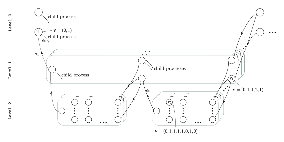
The state-expanded hypergraph of the first stage of a hierarchical MDP. Level 0 indicate the founder level, and the nodes indicates states at the different levels. A child process (oval box) is represented using its state-expanded hypergraph (hyperarcs not shown) and is uniquely defined by a given state and action of its parent process.
Since a child process is always defined by a stage, state and action of the parent process we have that for instance a state at Level 1 can be identified using an index vector where is the state id at the given stage in the process defined by the action in state at stage . Note all values are ids starting from zero, e.g. if it is the first state at the corresponding stage and if it is the third action at the corresponding state. In general a state and action at level can be uniquely identified using The index vectors for state , and are illustrated in the figure. As under a semi-MDP another way to identify a state in the state-expanded hypergraph is using an unique id.
Example
Let us try to solve a small problem from livestock farming, namely the cow replacement problem where we want to represent the age of the cow, i.e. the lactation number of the cow. During a lactation a cow may have a high, average or low yield. We assume that a cow is always replaced after 4 lactations.
In addition to lactation and milk yield we also want to take the genetic merit into account which is either bad, average or good. When a cow is replaced we assume that the probability of a bad, average or good heifer is equal.
We formulate the problem as a HMDP with 2 levels. At level 0 the
states are the genetic merit and the length of a stage is a life of a
cow. At level 1 a stage describe a lactation and states describe the
yield. Decisions at level 1 are keep or
replace.
Note the MDP runs over an infinite time-horizon at the founder level where each state (genetic merit) define a semi-MDP at level 1 with 4 lactations.
Let us try to load the model and get some info:
prefix <- paste0(system.file("models", package = "MDP2"), "/cow_")
mdp <- load_mdp(prefix)
#> Read binary files (0.000313733 sec.)
#> Build the HMDP (0.000186195 sec.)#> Checking MDP and found no errors (4.917e-06 sec.)
mdp#> $bin_names
#> [1] "/home/runner/work/_temp/Library/MDP2/models/cow_stateIdx.bin"
#> [2] "/home/runner/work/_temp/Library/MDP2/models/cow_stateIdxLbl.bin"
#> [3] "/home/runner/work/_temp/Library/MDP2/models/cow_actionIdx.bin"
#> [4] "/home/runner/work/_temp/Library/MDP2/models/cow_actionIdxLbl.bin"
#> [5] "/home/runner/work/_temp/Library/MDP2/models/cow_actionWeight.bin"
#> [6] "/home/runner/work/_temp/Library/MDP2/models/cow_actionWeightLbl.bin"
#> [7] "/home/runner/work/_temp/Library/MDP2/models/cow_transProb.bin"
#> [8] "/home/runner/work/_temp/Library/MDP2/models/cow_externalProcesses.bin"
#> [9] "/home/runner/work/_temp/Library/MDP2/models/cow_transWeight.bin"
#> [10] "/home/runner/work/_temp/Library/MDP2/models/cow_transWeightLbl.bin"
#>
#> $time_horizon
#> [1] Inf
#>
#> $states
#> [1] 42
#>
#> $founder_states_last
#> [1] 3
#>
#> $actions
#> [1] 69
#>
#> $levels
#> [1] 2
#>
#> $weight_names
#> [1] "Duration" "Net reward" "Yield"
#>
#> $weight_action_names
#> [1] "Duration" "Net reward" "Yield"
#>
#> $weight_trans_names
#> character(0)
#>
#> $ptr
#> C++ object <0x564ab8913680> of class 'HMDP' <0x564abb4a0480>
#>
#> attr(,"class")
#> [1] "HMDP" "list"The state-expanded hypergraph representing the HMDP with infinite time-horizon can be plotted using
hgf <- get_hypergraph(mdp)
## Rename labels
dat <- hgf$nodes %>%
  dplyr::mutate(label = dplyr::case_when(
    label == "Low yield" ~ "L",
    label == "Avg yield" ~ "A",
    label == "High yield" ~ "H",
    label == "Dummy" ~ "D",
    label == "Bad genetic level" ~ "Bad",
    label == "Avg genetic level" ~ "Avg",
    label == "Good genetic level" ~ "Good",
    TRUE ~ "Error"
  ))
## Set grid id
dat$g_id[1:3] <- 85:87
dat$g_id[43:45] <- 1:3
get_g_id <- function(process, stage, state) {
  if (process == 0) start <- 18
  if (process == 1) start <- 22
  if (process == 2) start <- 26
  return(start + 14 * stage + state)
}
idx <- 43
for (process in 0:2) {
  for (stage in 0:4) {
    for (state in 0:2) {
      if (stage == 0 & state > 0) break
      idx <- idx - 1
      # cat(idx,process,stage,state,get_g_id(process,stage,state),"\n")
      dat$g_id[idx] <- get_g_id(process, stage, state)
    }
  }
}
hgf$nodes <- dat
## Rename labels
dat <- hgf$hyperarcs %>%
  dplyr::mutate(
    label = dplyr::case_when(
      label == "Replace" ~ "R",
      label == "Keep" ~ "K",
      label == "Dummy" ~ "D",
      TRUE ~ "Error"
    ),
    col = dplyr::case_when(
      label == "R" ~ "deepskyblue3",
      label == "K" ~ "darkorange1",
      label == "D" ~ "black",
      TRUE ~ "Error"
    ),
    lwd = 0.5,
    label = ""
  )
hgf$hyperarcs <- dat
## Make the plot
plot_hypergraph(hgf, grid_dim = c(14, 7), cex = 0.8, radx = 0.02, rady = 0.03)
Note action keep is drawn with orange color and action
replace with blue color.
We find the optimal policy under the expected discounted reward criterion using policy iteration with an interest rate of 10%:
w_lbl <- "Net reward" # the weight we want to optimize (net reward)
dur_lbl <- "Duration" # the duration/time label
run_policy_ite_discount(mdp, w_lbl, dur_lbl, rate = 0.1)
#> Run policy iteration using weight 'Net reward' under discounted expected-weight Bellman operator
#> with 'Duration' as duration using discount factor 0.904837.
#> Iteration(s): 1 2 3 4 finished. Cpu time: 4.917e-06 sec.The optimal policy is:
hgf$hyperarcs <- right_join(hgf$hyperarcs, get_policy(mdp), by = c("s_id", "a_idx"))
plot_hypergraph(hgf, grid_dim = c(14, 7), cex = 0.8, radx = 0.02, rady = 0.03)
We may also find the policy which maximize the average reward per lactation:
w_lbl <- "Net reward" # the weight we want to optimize (net reward)
dur_lbl <- "Duration" # the duration/time label
run_policy_ite_ave(mdp, w_lbl, dur_lbl)
#> Run policy iteration under average expected-weight Bellman operator using
#> weight 'Net reward' over 'Duration'. Iterations (g):
#> 1 (11000) 2 (11517.5) 3 (11543.8) 4 (11543.8) finished. Cpu time: 4.917e-06 sec.#> [1] 11543.83
get_policy(mdp)#> # A tibble: 42 × 6
#> s_id state_str state_label a_idx action_label weight
#> <dbl> <chr> <chr> <int> <chr> <dbl>
#> 1 3 0,2,0,4,0 Low yield 0 Replace -7369.
#> 2 4 0,2,0,4,1 Avg yield 0 Replace -5369.
#> 3 5 0,2,0,4,2 High yield 0 Replace -3369.
#> 4 6 0,2,0,3,0 Low yield 0 Keep -5912.
#> 5 7 0,2,0,3,1 Avg yield 0 Keep -2912.
#> 6 8 0,2,0,3,2 High yield 0 Keep 87.7
#> 7 9 0,2,0,2,0 Low yield 0 Keep -3956.
#> 8 10 0,2,0,2,1 Avg yield 0 Keep -456.
#> 9 11 0,2,0,2,2 High yield 0 Keep 3044.
#> 10 12 0,2,0,1,0 Low yield 0 Keep -3750.
#> # ℹ 32 more rowsSince other weights are defined for each action we can calculate the average reward per litre milk under the optimal policy:
run_calc_weights(mdp, w = w_lbl, criterion = "average", dur = "Yield")#> [1] 1.932615or the average yield per lactation:
run_calc_weights(mdp, w = "Yield", criterion = "average", dur = dur_lbl)#> [1] 5973.166